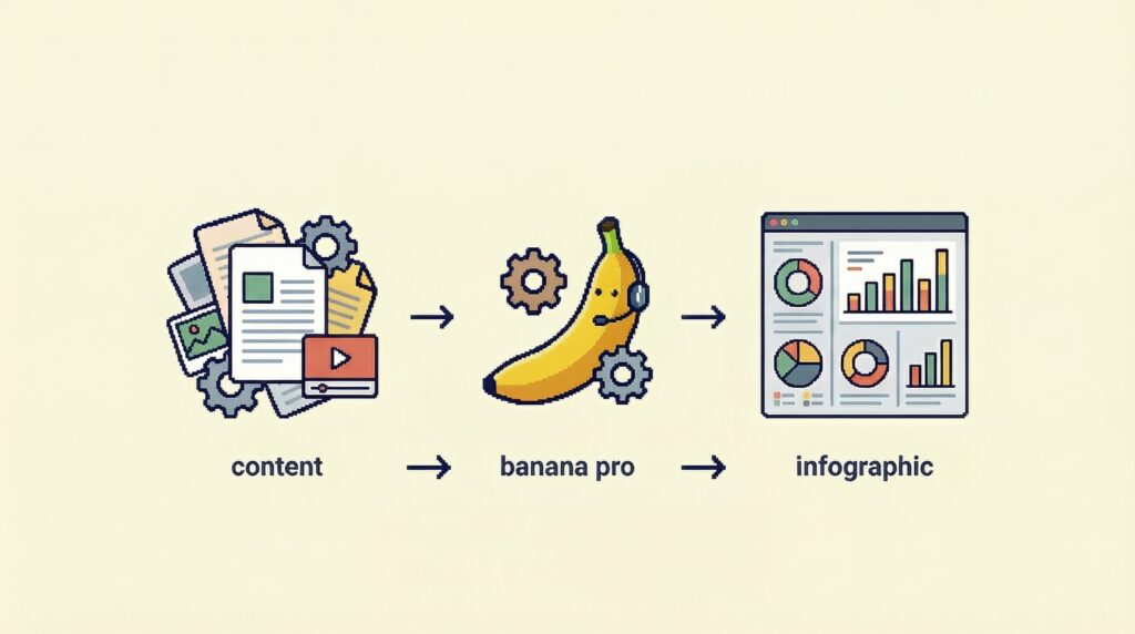
Create Stunning Infographics using Nano Banana Pro in Agentic Way
More
Introduction Forget the old times when you had to manually create infographics. With Nano Banana Pro, you can now create stunning infographics in minutes. Nano Banana Pro is an advanced AI image generation and editing model developed by Google DeepMind as part of the Gemini AI family. It’s essentially a professional grade tool for creating high-quality visuals—like illustrations, infographics, mockups, and edited photos using natural language text prompts or reference images. In this blog post, we will build a web application that leverages Nano Banana Pro to generate stunning infographics from any accessible content such as articles, and store the generated infographics data using GridDB as the high-performance database backend. Running the Application To run this application, you need to: Clone this repository and run the following commands: $ git clone https://github.com/junwatu/infographic-nbp-griddb.git $ cd infographic-nbp-griddb/apps $ npm install Set up the environment variables. Copy the .env.example file to .env and fill in the values: $ WEB_URL=http://localhost:3000 $ # GridDB Web API Configuration (Primary) $ GRIDDB_WEBAPI_URL="" $ GRIDDB_USERNAME="" $ GRIDDB_PASSWORD="" $ # DeepSeek API key through Anthropic-compatible endpoint $ NEBIUS_API_KEY="" $ # Nano Banana Pro through Fal API $ FAL_KEY="" Start the application: $ npm run dev Open http://localhost:3000 in your browser and paste an article URL to generate an infographic. Please note that the article should be publicly accessible from the internet and not behind a paywall. System Architecture A user submits an input through the browser, which is sent to a Node.js backend that contains two core components: a Content Retriever and a Prompt AI Agent (DeepSeek-V3.2). The Content Retriever enriches or contextualizes the user request (e.g., fetching references, templates, or prior data), after which the Prompt AI Agent constructs a structured prompt. The prompt, along with image metadata, is persisted to a GridDB database for future retrieval. The finalized prompt is then forwarded to an external image generation AI model, Nano Banana Pro, which produces the image artifact and stores it in a file system. The generated image is subsequently served back to the browser, closing the loop. Technologies Used Node.js This project is built using React + Vite, which requires Node.js version 16 or higher. You can download and install Node.js from nodejs.org. Nano Banana Pro API Key You need to create a Google API key to use the Nano Banana Pro. In this project we use FAL inference provider to access the Nano Banana Pro API. Please note that using the Nano Banana Pro API requires a paid subscription plan. DeepSeek-V3.2 API Key The latest version of DeepSeek model is V3.2, which is a recently released large language model (LLM) developed by the Chinese AI company DeepSeek, specifically optimized for coding, agentic workflows, and tool-use tasks rather than just general text chat. To use the DeepSeek-V3.2 API, you must obtain an API key from the Nebius Platform. Simply create an account and generate your key from the dashboard. Please note that an active subscription plan is required to access the API features. > The application uses the OpenAI Agents SDK which connects to DeepSeek-V3.2 via an OpenAI-compatible base URL. This is why the environment variable is named NEBIUS_API_KEY. GridDB Sign Up for GridDB Cloud Free Plan If you would like to sign up for a GridDB Cloud Free instance, you can do so at the following link: https://form.ict-toshiba.jp/download_form_griddb_cloud_freeplan_e. After successfully signing up, you will receive a free instance along with the necessary details to access the GridDB Cloud Management GUI, including the GridDB Cloud Portal URL, Contract ID, Login, and Password. GridDB WebAPI URL Go to the GridDB Cloud Portal and copy the WebAPI URL from the Clusters section. It should look like this: GridDB Username and Password Go to the GridDB Users section of the GridDB Cloud portal and create or copy the username for GRIDDB_USERNAME. The password is set when the user is created for the first time. Use this as the GRIDDB_PASSWORD. For more details, to get started with GridDB Cloud, please follow this quick start guide. IP Whitelist When running this project, please ensure that the IP address where the project is running is whitelisted. Failure to do so will result in a 403 status code or forbidden access. You can use a website like What Is My IP Address to find your public IP address. To whitelist the IP, go to the GridDB Cloud Admin and navigate to the Network Access menu. AI Agents This application uses a multi-agent architecture powered by the OpenAI Agents SDK with DeepSeek-V3.2 as the underlying language model. The system consists of two specialized agents that work together in a coordinated pipeline. Agent Architecture Content Fetcher Agent The Content Fetcher is a specialized agent responsible for retrieving and cleaning article content from URLs. It’s extract the main content from web pages, removing ads, navigation, and other clutter. const createContentAgent = (model: any) => { return new Agent({ name: "Content Fetcher", instructions: "You are an expert at fetching and cleaning article content from URLs.", model, tools: [fetchArticleTool], }); }; The fetchArticleTool internally calls the fetchAndSanitize function which: Fetches the HTML from the provided URL Parses it using JSDOM Extracts the main content using Readability Returns a simplified object containing the title and textContent to the agent. Infographic Orchestrator Agent The Orchestrator is the manager agent that coordinates the entire infographic generation pipeline. It has access to two tools: fetch_article – The Content Fetcher agent exposed as a tool image_generator – Generates images using Nano Banana Pro via Fal const createOrchestratorAgent = (model: any, contentAgent: Agent) => { return new Agent({ name: "Infographic Orchestrator", instructions: ` You are the manager of an infographic generation pipeline. Your goal is to take a URL, fetch the content, create a prompt, and finally generate an image. Follow these steps strictly: 1. Use 'fetch_article' to get the article content. 2. Generate a detailed infographic prompt based on that content. 3. Call 'image_generator' with the prompt to create the final image. `, model, tools: [ contentAgent.asTool({ toolName: "fetch_article", toolDescription: "Fetches article content from a URL.", }), imageGeneratorTool, ], }); }; The Pipeline Flow When generateInfographicForUrl(url) is called, the orchestrator executes the following pipeline: const result = await run( orchestratorAgent, `Follow the infographic pipeline for this article: ${url} Step 1: Fetch the article content. Step 2: Generate a detailed prompt for an infographic. Step 3: CALL the 'image_generator' tool with that prompt. (MANDATORY) Finally, return ONLY a breakdown as JSON in this format: { "title": "Article Title", "image": "The generated image URL", "article_url": "${url}", "description": "Short summary", "prompt": "The full detailed prompt you used for 'image_generator'" }`, { maxTurns: 10 } ); The result is a structured JSON object containing: Field Description title Article title image Generated infographic URL article_url Original article URL description Short summary prompt The full prompt used for image generation Prompt Engineering The key to generating high-quality infographics lies in the prompt engineering. The orchestrator agent is instructed to create a detailed infographic prompt based on the article content. This prompt should include: Key statistics and data points from the article Visual layout suggestions (sections, hierarchy) Color scheme recommendations Typography and iconography hints The main message or takeaway The DeepSeek-V3.2 model excels at this task because it’s specifically optimized for agentic workflows and tool-use, making it ideal for following the multi-step pipeline instructions reliably. GridDB Data Layer The application uses a layered approach for database operations, with two key files: griddb-base.ts for database configuration and griddb.ts for infographic-specific operations. Database Schema The infographic container stores generated infographic metadata: Column Type Description id INTEGER Unique record identifier (rowkey) prompt STRING AI prompt used for image generation infographic STRING URL of the generated image article_url STRING Source article URL generation_timestamp TIMESTAMP When the record was created Base Configuration The base module (griddb-base.ts) handles database initialization with retry support: export const GRIDDB_CONFIG: GridDBConfig = { griddbWebApiUrl: process.env.GRIDDB_WEBAPI_URL || '', username: process.env.GRIDDB_USERNAME || 'admin', password: process.env.GRIDDB_PASSWORD || 'admin', timeout: 30000, retryAttempts: 3, retryDelay: 1000 }; The module also provides ensureContainer() which automatically creates the container with the defined schema if it doesn’t exist during server startup. CRUD Operations The main GridDB module (griddb.ts) exposes these functions: Function Description getInfographics(limit) Retrieve records ordered by timestamp (default: 100) getInfographicById(id) Get a single record by ID deleteInfographic(id) Remove a record by ID > Note: The saveInfographic() function is demonstrated in the Generate Infographic & Save to GridDB section below. Server Side API Routes Method Endpoint Description Request Body GET /health Server health check N/A POST /generate-infographic Generate and save infographic from URL { “url”: “string” } POST /api/infographics Manually save infographic record Infographic Object GET /api/infographics Retrieve all infographic records N/A GET /api/infographics/:id Retrieve a specific record by ID N/A DELETE /api/infographics/:id Delete a specific record by ID N/A Generate Infographic & Save to GridDB There are few endpoints available for the server and the most used is /generate-infographic route. This route is used to generate an infographic from a URL and also save the record to GridDB. This route will call the generateInfographicForUrl function from the orchestrator, which is an AI agent that orchestrates the infographic generation pipeline. More on this later. const result = await generateInfographicForUrl(url); Then if the image generation is successful, the result will be saved to GridDB. try { await saveInfographic({ id: 0, // ID is generated inside saveInfographic prompt: result.prompt, infographic: result.image, article_url: result.article_url || url, generation_timestamp: new Date().toISOString() }); } catch (dbError) { console.error('[Server] Failed to save to GridDB, but continuing:', dbError); } > Please note that the infographic record is an image URL instead of the image itself. The server also provide manual save endpoint /api/infographics to save infographic record to GridDB using POST request. This is useful for testing and debugging. Get All Infographics The GET /api/infographics endpoint retrieves all infographic records from GridDB by calling the getInfographics() wrapper function. Test with curl: $ curl -s http://localhost:3000/api/infographics Get Infographic by ID The GET /api/infographics/:id endpoint retrieves a specific infographic record. It includes validation for the ID parameter and proper error handling: const id = parseInt(req.params.id); if (isNaN(id)) { return res.status(400).json({ error: 'Invalid ID format' }); } const data = await getInfographicById(id); if (!data) { return res.status(404).json({ error: 'Infographic not found' }); } res.json(data); Test with curl: $ curl -s http://localhost:3000/api/infographics/368368397 Delete Infographic by ID The DELETE /api/infographics/:id endpoint removes a specific infographic record from GridDB. It follows the same ID validation pattern as the GET endpoint, then calls deleteInfographic(id) to remove the record. Test with curl: $ curl -X DELETE http://localhost:3000/api/infographics/368368397 > All endpoints follow a consistent pattern: validate input, call the appropriate GridDB wrapper function, and return JSON responses with proper HTTP status codes. Client Side The frontend is built with React and Vite, providing a fast and responsive user interface for generating infographics. UI Components The application uses a set of reusable UI components located in src/components/ui/: Component Description Button Primary action button with loading state support Card Container component with header, content, and footer sections Input Text input field with icon support Skeleton Loading placeholder for content Application Flow The main App.tsx component manages the entire user interaction flow: 1. URL Input Users enter an article URL into the input field. The form submission triggers the handleGenerate function: const handleGenerate = async (e: React.FormEvent) => { e.preventDefault() setLoading(true) const response = await fetch('/generate-infographic', { method: 'POST', headers: { 'Content-Type': 'application/json' }, body: JSON.stringify({ url }), }) const data = await response.json() setResult(data.result) } 2. Loading State While the infographic is being generated, a skeleton loader is displayed with an animated message: {loading && ( <Skeleton className="h-[400px] w-full rounded-xl" /> <p className="animate-pulse">Analyzing content and generating visuals…</p> )} 3. Result Display Once generated, the infographic is displayed in a styled card with: Article title and description The generated infographic image Link to the original article Download button for the image {result && ( <Card> <CardHeader> <CardTitle>{result.title}</CardTitle> <CardDescription>{result.description}</CardDescription> </CardHeader> <CardContent> <img src={result.image} alt={result.title} /> </CardContent> <CardFooter> <a href={result.article_url}>Original Article</a> <Button>Download Image</Button> </CardFooter> </Card> )} 4. Error Handling If an error occurs during generation, a styled error card is displayed: {error && ( <Card className="border-destructive bg-destructive/10"> <CardTitle className="text-destructive">Error</CardTitle> <CardDescription>{error}</CardDescription> </Card> )} State Management The application uses React’s useState hook to manage four pieces of state: State Type Purpose url string The article URL entered by the user loading boolean Whether a generation is in progress result InfographicResult \ null The generated infographic data error string \ null Error message if generation fails Limitations This article is a proof of concept and may have limitations, such as: Does not handle paywall articles. Doesnt handle URL malformed articles, API limit exceeded, etc. References Nano Banana Pro Nebius
Creating a GridDB MCP Server for CRUD Operations
More
Modern AI systems increasingly rely on external tools, databases, and services, which makes interoperability a core requirement for building flexible
Building a Real-Time GridDB Dashboard for Factory Floor Monitoring
More
Modern factory floors continuously generate streams of sensor data, including temperature, humidity, vibration and how much they are producing. On their own, each reading might not seem important. When you collect this data from many machines over a long time it is the best way for a factory to find problems early and avoid shutting down for a long time. The main challenge is that this data is time-series: it is timestamped, arrives quickly, and is usually written once. Using a general-purpose relational table can work when there is not much data, but as you add more sensors and keep data longer, problems appear. Indexes get too large, range queries slow down, and deleting old data becomes difficult. This post walks through a complete solution: a Java application that simulates readings from three factory sensors, stores them in GridDB‘s native TimeSeries containers, and serves a live web dashboard that displays rolling averages and threshold alerts in real time. GridDB is an open-source distributed NoSQL database purpose-built for IoT and time-series workloads. Its TimeSeries containers are optimized for exactly the shape of problem a sensor fleet like this one produces: high write throughput paired with efficient temporal queries. — What you’ll learn By the end of this tutorial, you’ll be able to: Set up a complete GridDB + Java environment using Docker Compose, with no local installation required Ingest time-series sensor data using GridDB’s TimeSeries containers and the append() method Query and analyze data with built-in aggregations (AVG, MIN, MAX) and TQL, GridDB’s SQL-like query language Visualize live data with a dashboard featuring sparklines, range gauges, and an alert log Deploy a pipeline that works on Windows, Mac, and Linux without host-networking issues — Prerequisites Docker and Docker Compose (Docker Desktop, with the WSL2 backend enabled if you’re on Windows) Java 17 and Maven — only needed if you want to build or modify the Java app outside of Docker; the provided Dockerfile handles both automatically if you’re just running the demo Git, to clone the project repository No local GridDB installation is required — it runs entirely inside the Docker Compose stack — Project structure griddb-dashboard-demo/ ├── docker-compose.yml └── app/ ├── Dockerfile ├── pom.xml └── src/main/ ├── java/com/example/griddb/ │ ├── Main.java │ ├── GridDbConnection.java │ ├── SensorReading.java │ ├── SensorIngestor.java │ └── DashboardServer.java └── resources/ └── dashboard.html docker-compose.yml at the root wires the GridDB server and the Java app together on a shared Docker network. Everything under app/ is the Java side: the Dockerfile builds it, pom.xml declares the GridDB client dependency, and dashboard.html is the front end served directly by the Java app’s embedded HTTP server. — Why a time-series database here GridDB is built around two container types: Collection, for general keyed data, and TimeSeries, which uses the row’s timestamp as its key and is optimized for exactly this append-heavy, time-ordered access pattern. For a monitoring use case, that means two things fall out almost for free: Efficient aggregation over time windows. Asking “what was the average temperature for sensor 3 over the last 24 hours” is a single built-in aggregation call, not a hand-rolled GROUP BY over a timestamp column. Natural isolation per device. Each sensor gets its own TimeSeries container, so a burst of writes from one noisy machine doesn’t contend with reads against another. It is worth comparing this approach with a traditional relational database design. A common starting point for many IoT projects is to store all sensor readings in a single relational table containing columns such as device_id, timestamp, and the measured values, with indexes added to support time-range queries. While this approach works well for small-scale deployments, it becomes increasingly difficult to maintain as the number of devices, data ingestion rate, and retention period grow. As sensor data grows, traditional relational databases become increasingly difficult to manage. Every new reading requires index updates, time-range queries must search ever-larger tables, and removing historical data often requires costly delete operations or custom partitioning strategies. GridDB is designed to address these challenges. Its native TimeSeries containers optimize sequential writes and time-based queries, while built-in row expiration automatically removes outdated data based on configurable retention policies. This reduces database maintenance and simplifies application development, making GridDB well suited for large-scale Industrial IoT and real-time monitoring applications. GridDB Compared with PostgreSQL and InfluxDB Feature GridDB PostgreSQL InfluxDB Native Time-Series Support Yes Partial (via extensions such as TimescaleDB) Yes Horizontal Scaling Yes Primarily vertical (distributed extensions available) Yes Query Language TQL (SQL-like) SQL InfluxQL / Flux Designed for Time-Series & IoT Yes General-purpose database Yes ACID Transactions Yes Yes Limited* Official Java Support Official Java Client JDBC Official Java Client Docker Support Yes Yes Yes > \* InfluxDB provides durability and consistency for time-series workloads but does not implement full ACID transactional semantics across multiple records in the same way as traditional relational databases such as PostgreSQL. — Architecture The system has four main components: GridDB server — running in Docker, one container from the standard GridDB image. A Java ingestion process — seeds historical data, then keeps appending a new reading every few seconds per simulated device. An embedded HTTP API — built on the JDK’s built-in com.sun.net.httpserver, so there’s no extra web framework to configure. It exposes /api/stats, /api/alerts, and /api/history. A dashboard page — polls those endpoints and renders a fleet summary strip, per-device panels with live sparkline trend lines and range gauges, and an alarm log. Everything ships in one docker-compose.yml, so docker compose up –build gets a full GridDB cluster and the Java app talking to each other on a bridge network. The complete source — the Dockerfile, docker-compose.yml, and all Java classes — is on GitHub: dagmawit-sudo-cloud/griddb-dashboard-demo. Clone it now to follow along and run each step as you read. Data flow, end to end — Why Docker Docker packages both GridDB and the Java application into isolated containers, so the exact same setup runs the same way regardless of whether it’s on your laptop, a teammate’s machine, or a CI pipeline — no “works on my machine” gap between installing GridDB natively and getting the Java client to find it. It also sidesteps a real platform-specific headache: Docker Desktop on Windows and Mac doesn’t support host networking the way Linux does, so a Compose setup using a proper bridge network (as this one does) is the version that actually works cross-platform, rather than one that only works if you happen to be on Linux. — Modeling a sensor reading The Java side talks to GridDB through its official Java Client API — the same supported gridstore library GridDB documents for production use, not a community wrapper or a raw protocol implementation. Every device writes rows shaped like this: public class SensorReading { @RowKey Date timestamp; String deviceId; double temperature; double humidity; boolean alertTriggered; } The @RowKey annotation on timestamp is what tells GridDB this class belongs in a TimeSeries container rather than a plain Collection. alertTriggered is computed at write time rather than derived later — efficient to compute once, and it lets the alerts endpoint run a simple boolean filter instead of recomputing a threshold check on every poll. Connecting, with retry Docker Compose starts containers in parallel, so the Java app frequently comes up before GridDB is actually ready to accept connections. The connection helper handles that with a bounded retry loop instead of failing hard on the first attempt: Properties props = new Properties(); props.setProperty("notificationMember", notificationMember); props.setProperty("clusterName", clusterName); props.setProperty("user", user); props.setProperty("password", password); for (int attempt = 1; attempt <= maxAttempts; attempt++) { try { GridStore store = GridStoreFactory.getInstance().getGridStore(props); System.out.println("Connected to GridDB at " + notificationMember); return store; } catch (GSException e) { System.out.println("Attempt " + attempt + "/" + maxAttempts + ": GridDB not ready yet (" + e.getMessage() + "), retrying in 5s…"); Thread.sleep(5000); } } All four connection properties — notification member, cluster name, user, password — are read from environment variables set in docker-compose.yml, which keeps the same image usable across dev and staging without a rebuild. > Tip: GridDB’s cluster takes 30–60 seconds to form after container startup. The retry loop ensures your application connects reliably even if it starts before the database is ready. Packaging the Java app The Java side builds as a two-stage Docker image, so the final container doesn’t carry a Maven install around at runtime: FROM maven:3.9-eclipse-temurin-17 AS build WORKDIR /build COPY pom.xml . COPY src ./src RUN mvn -q clean package -DskipTests FROM eclipse-temurin:17-jre WORKDIR /app COPY –from=build /build/target/app.jar app.jar EXPOSE 8080 CMD ["java", "-jar", "app.jar"] The build stage compiles the fat jar with Maven; the runtime stage starts from a bare JRE image and copies only the finished artifact across. The net effect is a noticeably smaller image and a faster docker compose up on the second run, since Docker’s layer cache skips the Maven download step entirely as long as pom.xml hasn’t changed. docker-compose.yml wires this image up to the GridDB container on a dedicated bridge network and passes in the connection properties as environment variables, so the two containers can find each other by service name (griddb-server:10001) without any manual network configuration. — Generating and appending data The application supports two ingestion workflows: an initial historical data load to populate the dashboard and a continuous streaming process that appends new sensor readings as they are generated. public static void ingest(GridStore store, String deviceId, int readingCount, double baseTemp) throws GSException { TimeSeries<SensorReading> ts = store.putTimeSeries(deviceId, SensorReading.class); for (int i = 0; i < readingCount; i++) { ts.append(buildReading(deviceId, baseTemp, new Random())); } } append() is the right call for time-series writes specifically — it assumes rows arrive in increasing timestamp order and skips the row-key lookup a generic put() would do, which matters once you’re writing thousands of readings a minute across many devices. The continuous variant runs the same append() call on a daemon thread every three seconds per device. — Querying: aggregates and alerts The stats endpoint leans on GridDB’s built-in aggregation functions rather than pulling raw rows into Java and averaging them by hand: Date now = TimestampUtils.current(); Date oneDayAgo = TimestampUtils.add(now, -24, TimeUnit.HOUR); double avg = ts.aggregate(oneDayAgo, now, "temperature", Aggregation.AVERAGE).getDouble(); double min = ts.aggregate(oneDayAgo, now, "temperature", Aggregation.MINIMUM).getDouble(); double max = ts.aggregate(oneDayAgo, now, "temperature", Aggregation.MAXIMUM).getDouble(); The alerts endpoint uses GridDB’s TQL query language instead, since it’s a row filter rather than an aggregate: Query<SensorReading> query = ts.query("WHERE alertTriggered", SensorReading.class); RowSet<SensorReading> rows = query.fetch(); > TQL pitfall: For boolean fields, TQL allows conditions to be written directly as WHERE alertTriggered, which is the form used throughout this example. Both endpoints return hand-built JSON strings over the JDK’s embedded HttpServer. That’s a deliberate simplification for a demo of this size — swap in your JSON library and framework of choice once the endpoint list grows past two. API endpoints Method & route Purpose GET /api/health Basic liveness check GET /api/stats Per-device avg/min/max/reading count over the configured window GET /api/alerts The most recent threshold-breaching readings across all devices GET /api/history?device= The last 40 readings for one device, oldest first — powers the sparkline trend line GET / The dashboard HTML page itself — The dashboard The dashboard is implemented as a lightweight, static HTML page served directly by the Java application’s embedded HTTP server. The interface is designed to resemble an industrial control-room dashboard, providing operators with a clear, real-time view of factory conditions. Every five seconds, the dashboard requests the latest data from the REST API and updates the display with three key monitoring components: A fleet summary displays an overview of the monitored environment, including the number of active devices, the fleet-wide average temperature, and the current number of active alerts. Device Monitoring panels present a dedicated panel for each sensor, featuring a status indicator, the latest sensor reading, a sparkline showing recent temperature trends, and a min/max range gauge with a configurable alert threshold. An alarm log displays the most recent threshold breaches and presents a clear empty state when no alerts have been triggered. That five-second polling interval is a knob worth tuning in your own setup tighter for a control-room display, looser if you’re polling over a slow network link. A close-up of a single device panel, showing the sparkline trend line and the min/max range gauge with the alert threshold marker. — Running it docker compose up –build Then open http://localhost:8080. Within a few seconds the device panels populate with live readings and trend lines, and if the simulated readings cross the alert threshold (27.5°C in this example), rows start appearing in the alarm log. Terminal output of docker compose up –build completing successfully, showing GridDB’s cluster starting and the Java app connecting. docker ps showing both containers — griddb-server and griddb-java-app — up and running on the shared bridge network. Checking the API directly It’s worth hitting the endpoints on their own before trusting the dashboard, both to confirm the data looks right and as a sanity check while you’re adapting this to your own sensors: $ curl http://localhost:8080/api/stats # [{"deviceId":"factory_floor_sensor_01","avg":26.84,"min":24.02,"max":31.97,"count":118}, …] $ curl http://localhost:8080/api/alerts # [{"deviceId":"factory_floor_sensor_01","timestamp":"2026-07-01T14:22:09.441Z","temperature":29.13}, …] Because both routes set Access-Control-Allow-Origin: *, they’re also easy to point a separate front end or a tool like Grafana’s JSON API plugin at, if the bundled dashboard ends up being a placeholder for something more elaborate. — Conclusion GridDB’s native time-series support, high write throughput, and straightforward Docker integration make it a strong fit for factory monitoring: TimeSeries containers handle the append-heavy, time-ordered access pattern that sensor data naturally produces, without the index maintenance and partitioning work a general-purpose relational table would require at the same scale. The full source for this project — the five Java classes, Dockerfile, and docker-compose.yml — is available on GitHub: dagmawit-sudo-cloud/griddb-dashboard-demo. References GridDB Java API Reference – https://www.griddb.net/en/resources/griddb-java-api-reference/ GridDB GitHub Repository – https://github.com/griddb/griddb Docker Documentation – https://docs.docker.com/ Chart.js Documentation –

Finding GridDB Cloud’s Ingest Ceiling with Fluentd
More
Fluentd is one of the most widely deployed log collectors in the world, and log ingestion is one of the workloads GridDB was built for: high-volume, append-heavy, time-stamped data. In this article we wire the two together using the fluent-plugin-griddb output plugin and GridDB Cloud, and then keep increasing the ingestion rate until something gives. As a brief summary: one small VM went from 15,000 to 150,000 rows per second by changing a single buffer parameter, and when we then quadrupled the collector hardware to push past that, throughput barely moved. We found the ceiling, and the way it shows up is more interesting than the number itself: not errors, not rejections, but quiet backpressure. Along the way we’ll cover a realistic installation (the plugin targets an older Ruby, so there is some dependency archaeology involved), a small patch the plugin needs before its buffered mode works, the container schema gotchas that the Web API’s positional row format will happily punish you for, and a version-drift bug that dressed itself up as a TLS problem. Why Fluentd GridDB has steadily grown its connector ecosystem: Kafka, JDBC, Grafana, and a range of collection agents can all read from or write to GridDB, which means it usually slots into an existing data pipeline rather than demanding a new one. Fluentd is a natural addition to that list. It is the de facto standard for log collection in a lot of Kubernetes and traditional server environments, it has hundreds of input and parser plugins, and once events are flowing through it, pointing them at GridDB is a single block. Everything in this post talks to GridDB Cloud through its Web API: JSON rows over HTTPS; it works from anywhere without special client libraries, and, as the numbers below will show, with sensible batching it moves more data than most logging workloads will ever generate. Installation For installation, fluent-plugin-griddb targets Ruby 2.7 and Fluentd 1.12. Ruby 2.7 predates OpenSSL 3, which is what modern Ubuntu ships, so Ruby will not compile against the system OpenSSL. The fix is to build OpenSSL 1.1.1 from source into its own prefix, build Ruby 2.7.2 against it with rbenv, and then pin RubyGems, Bundler, and Fluentd to the last versions that still support Ruby 2.7. It sounds worse than it is; each step is mechanical. 1. System dependencies $ sudo apt update $ sudo apt install -y git curl build-essential libreadline-dev zlib1g-dev \ libyaml-dev libncurses5-dev libffi-dev libgdbm-dev 2. OpenSSL 1.1.1 from source $ cd /tmp $ wget https://www.openssl.org/source/openssl-1.1.1w.tar.gz $ tar xvfz openssl-1.1.1w.tar.gz $ cd openssl-1.1.1w $ ./config –prefix=/opt/openssl-1.1.1w –openssldir=/opt/openssl-1.1.1w shared zlib $ make -j$(nproc) $ sudo make install One step that is easy to miss: the freshly built OpenSSL has an empty certificate directory, so anything compiled against it will fail TLS verification, including HTTPS calls to GridDB Cloud. Point it at the system certificate store: $ sudo rm -rf /opt/openssl-1.1.1w/certs $ sudo ln -s /etc/ssl/certs /opt/openssl-1.1.1w 3. rbenv and Ruby 2.7.2 Install rbenv, but pull ruby-build directly from GitHub. The version definitions that come with the packaged rbenv are stale and may not build 2.7.2 cleanly: $ sudo apt install -y rbenv $ mkdir -p "$(rbenv root)"/plugins $ git clone https://github.com/rbenv/ruby-build.git "$(rbenv root)"/plugins/ruby-build $ RUBY_CONFIGURE_OPTS="–with-openssl-dir=/opt/openssl-1.1.1w" rbenv install 2.7.2 $ rbenv global 2.7.2 $ echo 'eval "$(rbenv init – bash)"' >> ~/.bashrc $ source ~/.bashrc $ ruby –version # should report 2.7.2 4. Fluentd and the plugin Ruby 2.7 also needs older RubyGems and Bundler; the current releases of both have dropped support. Pin them, then install Fluentd 1.12.0 and the plugin gem: $ gem update –system 3.4.22 $ gem install bundler -v 2.4.22 $ gem install fluentd –version "1.12.0" –no-doc $ rbenv rehash $ gem install –force –local fluent-plugin-griddb-1.0.2.gem $ rbenv rehash A quick fluentd –version confirms the pipeline pieces are in place. And make sure it is 1.0.2 of the plugin specifically; more on why in a moment. Patching the Plugin Version 1.0.2 of the plugin has a latent bug: it works in its default, unbuffered mode, but the moment you add a section to the match block (which you will want for any serious throughput), Fluentd switches the plugin to its buffered code path, and that path calls a method that does not exist: $ error_class=NoMethodError error="undefined method `handle_record' for #<Fluent::Plugin::GriddbOutput> Did you mean? handle_create_container" Inside out_griddb.rb, the unbuffered process path routes records through a method called handle_insert_type, which works. The buffered write(chunk) path calls handle_record, which was never implemented. Every chunk raises, gets flagged as a bad chunk, and is shunted to Fluentd’s backup directory. The fix is one line: make the buffered path call the same method the working path uses. $ sed -i 's/handle_record(record_array)/handle_insert_type(record_array)/' \ $ "$(gem which fluent/plugin/out_griddb)" Note the use of gem which to locate the file. If you have the plugin’s source repository checked out as well as the gem installed, it is easy to edit the wrong copy and wonder why nothing changed. gem which fluent/plugin/out_griddb tells you exactly which file Fluentd loads. Two related notes while we are in the plugin internals. First, the plugin’s insert_type parameter accepts single and multiple, but multiple is currently a stub that logs “Currently insert type only support for single type” and does nothing, so leave it on single. Second, and this matters for the results later: even in single mode, the buffered path sends an entire buffer chunk in one HTTP request. So batch size is controlled by the buffer’s chunk settings, not by the insert type. Creating the Target Container The Web API inserts rows positionally: each row arrives as an array of values, matched to columns strictly by order. That makes the container schema definition load-bearing in a way that name-based systems are not, and it produced two instructive failures before the schema below worked. The event we will generate has six fields, plus a seq counter that Fluentd’s sample input appends to the end of each record. Appends, as in: seq arrives as the last value in the row, so it must be the last column in the schema. Defining it first produces The specified data cannot be converted to LONG type as the host string lands in the seq slot. Defining extra columns the record does not send (say, copying the schema of an apache-parsed container with user and referer fields) produces Row data is invalid from the value-count mismatch. The schema that matches what the plugin actually sends: $ curl -X POST \ $ -u "$GRIDDB_USER:$GRIDDB_PASS" \ $ -H 'Content-Type: application/json' \ $ "$GRIDDB_WEBAPI_URL/dbs/$GRIDDB_DB/containers" \ $ -d '{ $ "container_name": "fluentdStress", $ "container_type": "COLLECTION", $ "rowkey": false, $ "columns": [ $ {"name": "host", "type": "STRING"}, $ {"name": "method", "type": "STRING"}, $ {"name": "path", "type": "STRING"}, $ {"name": "code", "type": "INTEGER"}, $ {"name": "size", "type": "INTEGER"}, $ {"name": "agent", "type": "STRING"}, $ {"name": "seq", "type": "LONG"} $ ] $ }' Or you can use the GridDB Cloud CLI Tool: griddb-cloud-cli create -i. We use a COLLECTION with rowkey false rather than a time-series container on purpose. A time-series container upserts on duplicate timestamps, and at tens of thousands of rows per second many events share a millisecond. A throughput test against a time-series container without a carefully unique key silently measures overwrites while reporting success. A rowkey-less collection accepts every insert as a distinct row, which is what we want to count. The Stress Configuration For a throughput test, tailing a log file written by a generator makes the generator and the disk the bottleneck. Fluentd’s built-in sample input creates events in memory instead, which lets us dial the input rate directly: $ <system> $ workers 4 # match your core count $ </system> $ <source> $ @type sample $ tag stress.griddb $ size 200 # events per emit $ rate 50000 # events per second $ auto_increment_key seq # unique trailing counter per event $ dummy {"host":"10.0.0.1","method":"GET","path":"/api/v1/users","code":200,"size":4096,"agent":"gridstress/1.0"} $ </source> $ <match stress.griddb> $ @type griddb $ host "$GRIDDB_CLOUD_HOST" $ cluster "$GRIDDB_CLUSTER" $ database "$GRIDDB_DB" $ container "fluentdStress" $ insert_mode "append" $ insert_type "single" $ username "$GRIDDB_USER" $ password "$GRIDDB_PASS" $ <buffer> $ @type memory $ chunk_limit_records 50000 # rows per HTTP request: the knob that matters $ chunk_limit_size 64MB $ flush_thread_count 8 $ flush_mode interval $ flush_interval 1s $ flush_thread_interval 0.1 $ total_limit_size 4GB $ retry_max_times 3 $ retry_type periodic $ retry_wait 1s $ overflow_action throw_exception $ </buffer> $ </match> The parameters worth understanding: chunk_limit_records sets how many rows travel in each PUT to the Web API, flush_thread_count sets how many of those requests run in parallel, and workers in the system block spreads the whole pipeline across CPU cores. Everything else is safety plumbing: total_limit_size bounds the memory buffer, and overflow_action throw_exception makes backpressure loud instead of silent, which is exactly what you want when the point of the exercise is to see what breaks. Measuring Fluentd’s own logs tell you what it sent; they do not tell you what the database kept. The only number that counts is the row count in the container, so we sample it and compute the delta over the actual elapsed time: $ A=$(griddb-cloud-cli sql query -s "select count(*) from fluentdStress" \ $ | grep -o '"Value":[0-9]*' | grep -o '[0-9]*'); T1=$(date +%s) $ sleep 60 $ B=$(griddb-cloud-cli sql query -s "select count(*) from fluentdStress" \ $ | grep -o '"Value":[0-9]*' | grep -o '[0-9]*'); T2=$(date +%s) $ echo "confirmed rows/sec: $(( (B – A) / (T2 – T1) ))" One measurement lesson learned the hard way: divide by real elapsed time, not the interval you asked for. Once the container holds tens of millions of rows, count(*) itself takes several seconds, and a sampler that assumes its nominal interval will overstate throughput badly. And confirmed rows per second, measured at the destination, is the honest metric. If Fluentd claims success while this number lags what was sent, rows are being dropped somewhere. In our runs that gap never appeared: everything sent was stored. Round One: Batch Size Is the Whole Game All single-node runs use the same event shape. The only variables changed between runs are the chunk size and the worker count. chunk_limit_records workers node(s) sustained rows/sec 5,000 1 1 x 2-core ~15,000 20,000 2 1 x 2-core ~116,000 50,000 2 1 x 2-core ~150,000 The leap from 15k to 150k comes almost entirely from batching. Per-request overhead, HTTP, TLS, JSON framing, is fixed cost; the more rows amortize it, the closer you get to the pipeline’s real capacity. And do the request math: at 150,000 rows per second in 50,000-row chunks, the client is making roughly three HTTP requests per second. This resolves a confusion that comes up constantly with cloud database quotas: platform limits are typically expressed against requests and connections, not rows, and a well-batched pipeline moves enormous row volume through a trickle of requests. Row throughput and request rate are independent axes. Round Two: More Hardware, Same Ceiling To push the ingestion even further, we figured would throw in more cores and more nodes. So: two VMs, 4 cores each, 4 Fluentd workers each, identical configs, both writing to the same container. Eight workers across eight cores, four times the collector CPU that produced the 150k number. Setting up the second node produced a bug worth recounting, because it disguised itself well. The second machine’s Fluentd immediately failed every request with: 400 The plain HTTP request was sent to HTTPS port Microsoft-Azure-Application-Gateway/v2 The configs were byte-identical. OpenSSL versions matched. Certificate symlinks matched. No proxy variables anywhere. The actual cause: gem install fluent-plugin-griddb without a version pin had installed 1.0.1 on the new box instead of 1.0.2, and 1.0.1 handles the URL scheme differently, quietly speaking plaintext HTTP to port 443. A minor plugin version drift between two “identical” nodes produced what looked exactly like a TLS or gateway misconfiguration. Pin your plugin versions across a fleet. And remember that reinstalling the gem also wipes the handle_record patch, which must be reapplied on every fresh install. With both nodes on patched 1.0.2, the combined result over a sustained run: configuration total collector cores sustained rows/sec (combined) 1 node, 2 cores 2 ~150,000 2 nodes, 4 cores each 8 ~168,000 Quadrupling collector capacity bought about 12%. That flatline is the signature of a shared ceiling downstream of the collectors: somewhere in GridDB Cloud’s ingest path, whether the database engine or the Azure Application Gateway fronting it, the pipeline saturates around 150-170k rows per second on this plan. What the Ceiling Looks Like Here is the part that matters for anyone running this in production: the ceiling does not announce itself with errors. There were no 429s, no 503s, no failed inserts, no dropped rows at any point. Every single request returned success. What changed was latency. Buffer flushes that normally complete in about a second began taking 20 to 29 seconds: $ [warn]: #1 buffer flush took longer time than slow_flush_log_threshold: $ elapsed_time=26.086 slow_flush_log_threshold=20.0 $ [warn]: #2 buffer flush took longer time than slow_flush_log_threshold: $ elapsed_time=27.094 slow_flush_log_threshold=20.0 $ [warn]: #3 buffer flush took longer time than slow_flush_log_threshold: $ elapsed_time=28.739 slow_flush_log_threshold=20.0 Under sustained saturation, throughput oscillates between roughly 120k and 190k rows per second as flush queues build and drain. GridDB Cloud applies backpressure by slowing acceptance, not by rejecting requests. That is graceful behavior, nothing is lost, but it has a monitoring consequence: an alerting setup that watches only error rates will report a perfectly healthy pipeline while ingest latency has grown by 25x. Watch flush duration, not just status codes. Conclusion & Takeaways Tune the buffer before anything else. The difference between a naive Fluentd-to-GridDB config and a tuned one is an order of magnitude, and it is almost entirely chunk_limit_records. If your pipeline feels slow, your batches are almost certainly too small. One well-tuned node covers most workloads. A single 2-core VM sustained 150,000 rows per second. Before scaling out collectors, check whether you are anywhere near that; most logging workloads are not. The ceiling is real, and it is polite. Around 150-170k rows per second on this plan, the ingest path saturates regardless of collector count. It degrades by latency, not by error, so monitor flush duration. Sent and stored never diverged: even at saturation, nothing was dropped. Pin plugin versions across nodes. A one-patch-version drift between two collectors produced a protocol-level failure that looked like a TLS misconfiguration. Fleet consistency is not optional. Measure at the destination, against real elapsed time. count(*) deltas are the ground truth, and they get slow as the container grows; divide by actual seconds or your numbers flatter you. The Web API, for its part, holds up incredibly well. JSON over HTTPS carries overhead, and the native transport would spend fewer cycles per row. But sustaining 150,000+ rows per second, error-free, through the least exotic interface imaginable is more ingest than the vast majority of logging workloads will ever need. We set out to break GridDB Cloud, and the closest we got was making it take a little longer to say
Comparing GridDB and TimescaleDB
More
If you are choosing an open source time series database to run on your own infrastructure, GridDB and TimescaleDB are two of the strongest candidates — and they take fundamentally different approaches. GridDB is a purpose-built time series database designed from the ground up for IoT-scale ingestion. TimescaleDB is a PostgreSQL extension that adds time series capabilities to a general-purpose relational database. For most, GridDB is the better choice for high-volume IoT and sensor workloads. But TimescaleDB is a genuinely good database, and there are workloads where it can be the correct choice. A note on scope: this comparison is GridDB Community Edition vs the open source edition of TimescaleDB At a Glance GridDB Community Edition TimescaleDB Current version 5.9 2.27 (May 2026) Vendor Toshiba TigerData (formerly Timescale Inc.) Architecture Purpose-built time series database, in-memory-first with disk persistence PostgreSQL extension (hypertables on top of Postgres) Data model Key-Container (Collection + TimeSeries containers) Relational tables, partitioned into hypertables/chunks Query interfaces NoSQL API (TQL) + SQL (JDBC) Full PostgreSQL SQL Horizontal scale-out (free edition) No — Community Edition is single-node; multi-node clustering is Enterprise Edition (commercial) No — multi-node was removed in v2.14; single-node only (scale-out via managed Tiger Cloud) High availability (free edition) No — clustering and failover are Enterprise Edition features Via external PostgreSQL replication tooling (Patroni, streaming replication) Compression Built-in time series compression, in the open source edition Columnstore compression — Timescale License (TSL) only, not in the Apache 2 edition Continuous aggregates / rollups Aggregation via TQL/SQL Continuous aggregates — TSL only License Server: AGPL v3 · Client libraries: Apache 2.0 Apache 2.0 (core) · TSL (source-available) for most advanced features Ecosystem GridDB clients (Java, Python, C, Go, Node.js, PHP), Kafka Connector, Grafana plugin The entire PostgreSQL ecosystem Best for Purpose-built high-cardinality IoT ingestion with advanced features under genuine open source Teams already on PostgreSQL, mixed relational + time series workloads Architecture: Purpose-Built vs Extension This is the most important difference, and a lot else flows from it. GridDB was designed by Toshiba specifically for IoT telemetry. Its architecture is in-memory-first — memory is the primary store and disk is secondary — with an event-driven engine designed to minimize overhead per operation. Data is organized into containers, and in a clustered deployment (Enterprise Edition) distributed across nodes automatically. The database was built assuming millions of devices writing high-frequency data, and the design decisions reflect that. TimescaleDB inherits PostgreSQL’s architecture: a row-oriented, disk-first, general-purpose relational engine. The extension adds hypertables — tables transparently partitioned into time-based chunks — plus a columnar compression engine for older data. This is a clever design that gets impressive results out of Postgres, but it is fundamentally an adaptation of an OLTP database to a time series workload, not a ground-up time series engine. The practical consequence: GridDB’s hot path for sensor ingestion (append a timestamped row to a TimeSeries container, in memory) is shorter than TimescaleDB’s (full PostgreSQL write path — WAL, MVCC bookkeeping, buffer management). For write-heavy IoT workloads, that architectural difference shows up in throughput and resource efficiency. The flip side: PostgreSQL’s general-purpose engine means TimescaleDB handles things GridDB doesn’t try to — complex multi-table joins, foreign keys against relational business data, window functions across arbitrary tables, and the full breadth of SQL. Data Model: Key-Container vs Hypertables GridDB uses a Key-Container model. Each data source — typically each sensor or device — gets its own container, addressed by key. TimeSeries containers treat the timestamp as the row key and provide time-specific operations (sampling, interpolation, time-window aggregation) natively. This maps one-to-one onto how real IoT systems are structured: a fleet of devices, each with its own schema and stream. Locating one device’s data never requires scanning an index shared with a million other devices. TimescaleDB keeps the relational model: all sensors typically write into one wide hypertable with a device ID column, and chunks partition it by time. This is comfortable if you think in SQL, and it makes cross-device analytical queries natural. The trade-off is that per-device access patterns compete inside shared structures, and schema differences between device types get awkward (sparse columns, JSONB, or table sprawl). Which model is better depends on your access pattern. Per-device reads and writes at high cardinality favor GridDB’s model. Ad-hoc analytics across all devices favor the relational model. Scalability: Both Free Editions Are Single-Node TimescaleDB’s multi-node support was deprecated and removed in version 2.14 (early 2024). Self-hosted TimescaleDB today is a single-node database: you scale by buying a bigger machine, and TigerData’s path to horizontal scale is their managed Tiger Cloud service. GridDB is the same story on the open source side: Community Edition runs as a single node, and multi-node clustering — automatic data partitioning, replication, and failover — is reserved for the commercial GridDB Enterprise Edition (and GridDB Cloud). So basically, we recommend you choose your free edition on single-node merits, and treat clustering as a separate, paid decision for both. A single GridDB node is less limiting than it sounds — its hybrid memory-and-disk design supports very large datasets (on the order of tens of terabytes per node) — and the same vertical-scaling logic applies to a single large TimescaleDB node. The meaningful open source difference is what each gives you within that single node, which is where licensing comes in. Licensing: Where the Open Source Editions Really Differ Neither database is “just open source,” and the difference here is the crux of the open source comparison. TimescaleDB ships in two editions. The Apache 2 edition is genuinely permissive open source — but it excludes most of what makes TimescaleDB compelling. Columnstore compression, continuous aggregates, and many recent performance features are part of the Community Edition, licensed under the Timescale License (TSL). The TSL is source-available, not OSI open source: it’s free to use as long as you are not offering TimescaleDB as a hosted database service, but it is a proprietary license with usage restrictions. In practice, the TimescaleDB you read about in benchmarks — compressed, with continuous aggregates — means accepting the TSL. GridDB Community Edition licenses the server under AGPL v3 and the client libraries under Apache 2.0, and — importantly — its advanced features, including built-in time series compression, are part of that open source edition. AGPL is a true OSI-approved open source license, though a strong copyleft one: if you modify the GridDB server and offer it as a network service, you must publish your modifications. For the overwhelmingly common case — running GridDB unmodified as the database behind your application, talking to it through the Apache 2.0 client libraries — AGPL imposes no obligations on your application code. Organizations with blanket AGPL bans should note this; everyone else will find it a non-issue. To summarize: GridDB CE gives you a purpose-built time series engine with its advanced features under an OSI open source license. TimescaleDB’s truly-open Apache edition is feature-limited, and its full capability is source-available (TSL) rather than open source. That — not clustering — is where GridDB’s free edition pulls ahead. Performance Both databases are fast, and both vendors publish benchmarks that favor themselves — including us. Rather than quote numbers here, we’ll note the architectural expectations and point you to reproducible tests. GridDB’s in-memory-first design and per-container data layout favor high-frequency ingestion and per-device range scans — the core IoT pattern. TimescaleDB’s columnstore compression and vectorized execution (significantly expanded in the 2.26–2.27 releases) favor analytical scans over compressed historical data. The Time Series Benchmark Suite (TSBS) supports both databases, and we encourage you to run it against your own workload shape — benchmark results vary enormously with cardinality, batch size, and query mix. TSDB_Evaluation_of_GridDB_QuestDB_and_TimescaleDB Ecosystem and Operations TimescaleDB wins on ecosystem. It is PostgreSQL, so every Postgres driver, ORM, BI tool, backup utility, monitoring exporter, and DBA skill set applies directly. If your team already runs Postgres, the operational learning curve is nearly zero. GridDB’s ecosystem is smaller but covers the IoT stack well: official clients for Java, Python, C, Go, Node.js, and PHP; a Kafka Connector for streaming pipelines; a Grafana plugin for visualization; and integrations with Telegraf, Fluentd, and Logstash for telemetry collection. Operationally, GridDB requires learning its own tooling — there is no equivalent of the Postgres DBA talent pool. When to Choose Which Choose GridDB if: Your workload is high-frequency sensor/IoT ingestion at high device cardinality You want a purpose-built time series engine rather than an extension on a general-purpose database You want advanced features like compression under a genuine open source license, not a source-available one You value having both a fast NoSQL (TQL) path and SQL (JDBC) access to the same data Choose TimescaleDB if: Your team already runs PostgreSQL and values that ecosystem above all Your workload mixes relational business data with time series and needs rich joins between them You’re comfortable with the TSL for compression and continuous aggregates, or plan to use Tiger Cloud A note on scale for both: if you outgrow a single node, horizontal clustering is a paid step either way — GridDB Enterprise Edition on one side, Tiger Cloud on the other. Factor that into a long-term decision rather than assuming the free edition will scale out. FAQ Is TimescaleDB still open source? Partially. The Apache 2 edition is open source but excludes columnstore compression, continuous aggregates, and most advanced features. The full-featured Community Edition uses the Timescale License (TSL), which is source-available but not OSI open source. Timescale Inc. rebranded as TigerData in June 2025. Can free TimescaleDB run as a cluster? No. Multi-node support was removed in TimescaleDB 2.14. Self-hosted TimescaleDB is single-node; horizontal scale requires their managed Tiger Cloud service. Can free GridDB run as a cluster? No. GridDB Community Edition runs as a single node. Multi-node clustering, replication, and failover are features of the commercial GridDB Enterprise Edition (and GridDB Cloud). Is GridDB SQL-compatible? Yes — GridDB provides a SQL interface via JDBC (its NewSQL interface) alongside its NoSQL API (TQL), and both are available in the open source Community Edition. Its SQL dialect is not as comprehensive as PostgreSQL’s, which is the trade-off for its purpose-built engine. Which is faster? It depends on workload shape. GridDB’s architecture favors high-frequency ingestion and per-device queries; TimescaleDB’s compression favors analytical scans of historical data. Run TSBS against your own workload — both databases support it. GridDB Community Edition is free and open source. Download it from GitHub or get started with the quick start
Comparing GridDB & MongoDB for Time Series Data
More
If you are choosing a database for time series data, GridDB and MongoDB are two of the most established options. In 2026 they make a surprisingly different bargain with you. GridDB is a purpose-built time series database whose Community Edition can query and analyze your full data history. MongoDB is a general-purpose document database that added native time series collections in version 5.0, keeping the document model and the rest of the MongoDB feature set available alongside them. We took GridDB Community Edition and MongoDB Community Server, ran through the workloads that matter to ingest, retention, and query history, and this page lays out the differences honestly so you can decide for yourself. A note on editions before we start. This comparison is primarily between GridDB Community Edition and MongoDB Community Server, since those are the two free, self-hosted, open source editions. Where the managed services (GridDB Cloud and MongoDB Atlas) change the answer, we say so. MongoDB’s time series collections have been available since 5.0 and are in the Community edition, not held back for commercial tiers. At a Glance GridDB Community Edition MongoDB Community Server Vendor Toshiba MongoDB, Inc. Architecture Purpose-built time series database, in-memory-first with disk persistence General-purpose document database; time series collections stored in an internal bucketed format Data model Key-Container (Collection and TimeSeries containers), strongly typed BSON documents with a timeField and an optional metaField; flexible per-document schema Query interfaces NoSQL API (TQL) plus SQL-92 over JDBC/ODBC MongoDB Query API and aggregation pipeline; SQL is read-only and Atlas-only Time series functions Built-in time-weighted average, time-bucket aggregation, interpolated sampling $setWindowFields, $densify, $fill, $dateTrunc in the aggregation pipeline Updates to measurements Full. Standard row inserts, updates, and deletes Restricted. Updates can only match on and modify the metaField; no upserts Writes in transactions Supported No. Time series collections cannot be written to inside a transaction; reads are supported Horizontal scale-out (free edition) No. Community Edition is single-node; multi-node clustering is in the commercial Advanced Edition Yes. Replica sets and sharding are included in Community Server High availability (free edition) No. Clustering and failover are Advanced Edition features Yes. Replica sets provide HA in the free edition Expiry (TTL) Yes, via expiration settings on the container Yes, via expireAfterSeconds Secondary indexes Yes, on container columns Yes, on any field since 6.0; compound metaField and timeField index created automatically Geospatial Native GEOMETRY type with spatial index and WKT, via the NoSQL interface GeoJSON with 2dsphere indexing, well established across the product License Server: AGPL v3 · Clients: Apache 2.0 SSPL for the server; drivers under Apache 2.0 Ecosystem GridDB clients (Java, Python, C, Go, Node.js, Ruby, PHP, Perl), Kafka Connector, Grafana, Fluentd, Telegraf, MQTT, Node-RED, Apache Arrow Very large general-purpose ecosystem: official drivers for nearly every language, Atlas, Compass, BI Connector, Kafka Connector Best for SQL-based analytics on high-frequency IoT and sensor data, on-premises or at the edge Applications where time series is one workload among several and the schema varies per document Architecture: Purpose-Built vs General-Purpose Both databases are well-engineered. They optimize for different things. GridDB was designed by Toshiba specifically for IoT telemetry. Its storage engine, container model, and built-in functions all assume you are ingesting large volumes of timestamped data at high frequency and querying it by time. It runs an in-memory-first architecture, a hybrid of memory and disk, tuned for high write throughput on this kind of data. The design assumes high-frequency data from many devices, retained and queryable over time. MongoDB approaches time series as a specialized capability layered onto a flexible document store. When you create a time series collection, MongoDB organizes writes so that data from the same source is stored alongside other data points from a similar point in time, in an internally optimized bucketed format. Under the hood, MongoDB treats time series collections as writable non-materialized views backed by an internal collection. The practical consequence cuts both ways. MongoDB’s bucketing gives you real time series efficiency without giving up the document model, so one system can serve both your operational data and your telemetry. GridDB’s narrower focus means the whole engine, not a collection type within it, is built around the time series access pattern. Data Model: Key-Container vs Time Series Collections GridDB uses a Key-Container model. Each data source, typically a sensor or device, gets its own container, addressed by key. A TimeSeries container uses a TIMESTAMP column as its row key. Data is strongly typed, which means schema is fixed up front and enforced. Through the SQL interface, a container is simply a table. MongoDB stores each measurement as a BSON document inside a time series collection. Each document carries a required timeField, an optional metaField identifying the source, and any number of measurement fields. The schema is flexible, so documents in the same collection can carry different fields entirely. The difference is clearest at creation time. MongoDB db.createCollection("sensors", { timeseries: { timeField: "timestamp", metaField: "sensorId", granularity: "seconds" }, expireAfterSeconds: 2592000 // auto-remove data after 30 days }) GridDB (SQL interface) CREATE TABLE sensors ( ts TIMESTAMP PRIMARY KEY, value DOUBLE ) USING TIMESERIES WITH (expiration_type='ROW', expiration_time=30, expiration_time_unit='DAY'); Which model suits you depends on your data. If every device emits the same fixed set of readings, GridDB’s typed containers give you enforcement and compactness. If your payloads vary by device generation, firmware version, or vendor, MongoDB’s per-document flexibility saves you from schema migrations. Query Interfaces: SQL vs Aggregation Pipeline This is often the deciding factor, and it is worth being precise because both databases are widely misdescribed here. GridDB offers two interfaces. TQL is a lightweight query language for the NoSQL side, and the SQL interface is SQL-92 compliant over standard JDBC and ODBC. A team that already knows SQL writes SELECT, JOIN, GROUP BY, and window queries without learning anything proprietary. The often-repeated claim that GridDB cannot do JOINs applies to TQL, not to the SQL interface. MongoDB uses its own Query API and aggregation pipeline rather than SQL, and for time series work it is genuinely capable. $setWindowFields gives you window functions such as moving averages and rank. $densify fills in missing time points and $fill populates their values by interpolation or carry-forward. $dateTrunc handles time bucketing for downsampling. The tradeoff is portability of skills and tooling. These are MongoDB-specific constructs, and a team standardized on SQL and SQL-based BI tools will face a learning curve. Atlas offers a read-only SQL interface for BI use cases, but that is a managed-service feature and it is read-only. The Update Restriction This is the difference that matters most between the two for operational workloads, and the one most likely to surprise people coming from a general-purpose MongoDB collection. MongoDB time series collections are designed around the assumption that telemetry is append-only. That assumption is enforced. Update commands must match only on the metaField value and can modify only the metaField value. Your update document can contain only update operator expressions, updates must be multi-document (multi: true or updateMany()), and upsert: true is not allowed. Deletes are supported and follow similar matching rules. Separately, you cannot write to a time series collection inside a multi-document transaction, though reads within transactions are supported. For a pure telemetry pipeline, none of this matters. Sensors emit readings, you never go back and edit them, and TTL handles the aging out. But a large share of real deployments do need corrections: a miscalibrated sensor whose readings need rescaling after the fact, a backfill that overwrites provisional values with settled ones, an ETL job that needs to be idempotent and therefore wants upserts. On MongoDB time series collections those patterns require a workaround, typically deleting and reinserting, or staging corrections in a separate regular collection. GridDB places no equivalent restriction on updating measurement values. If your workload involves in-place correction of individual readings, or writes that need to participate in transactions, test that path early on both databases rather than discovering it late. Scalability: Where the Free Editions Differ It is worth being precise here, because MongoDB has the advantage in the free edition and we would rather say so than have you find out later. MongoDB Community Server includes both replica sets and sharding. You get high availability and horizontal scale-out without paying for a commercial license. For time series collections specifically, the recommended practice is to include the metaField in the shard key so that data from the same source stays co-located. A few constraints apply: shard keys containing the timeField are deprecated as of 8.0, zone sharding is not supported for time series collections, and resharding a time series collection became available only in 8.0.10. MongoDB 8.0 also brought substantial improvements to sharding speed and cost. GridDB Community Edition is single-node. Multi-node clustering, replication, and automatic failover are part of the commercial Advanced Edition and of GridDB Cloud. The underlying architecture is a distributed shared-nothing design built for large-scale ingest, but you reach it through the commercial editions, not the free one. So if clustering or high availability on a zero-cost license is a hard requirement, MongoDB Community meets it and GridDB Community does not. If you are comparing commercial tier to commercial tier, both scale horizontally and the comparison comes back to workload fit. For either database, benchmark against a representative slice of your own workload rather than relying on general throughput claims. Results depend heavily on cardinality, batch sizes, and query patterns. Licensing GridDB ships the server under AGPL v3 with clients under Apache 2.0. AGPL imposes obligations on your application code: the copyleft only triggers if you modify the GridDB server itself and offer that modified server as a network service, but organizations with blanket AGPL bans should note this. Commercial Standard, Advanced, and Vector editions are available, as is the managed GridDB Cloud. MongoDB uses the SSPL for the server, with drivers under Apache 2.0. The SSPL is not an OSI-approved open source license, and it is more aggressive than AGPL in one specific direction: it targets organizations offering the database itself as a service. For the overwhelming majority of users, who are building an application on top of MongoDB rather than reselling MongoDB, it imposes no practical burden. But it has been enough to get MongoDB removed from some Linux distribution repositories, and some enterprise legal teams treat SSPL as disqualifying on principle. Neither license is a problem for a typical internal application. Both are worth a five-minute conversation with legal before you commit. Performance GridDB’s in-memory-first design and per-container layout favor high-frequency ingestion and per-device range scans across the full dataset. MongoDB’s bucketed storage format substantially narrows the gap against general-purpose document storage, and its compound metaField and timeField index serves the common “one source over a time window” query well. Rather than repeat vendor claims, we would point you at the published benchmark work and, more importantly, at your own workload. Cardinality, batch size, payload shape, and query mix move these numbers more than any architectural difference does. Ecosystem and Operations MongoDB wins on ecosystem breadth, and it is not close. Official drivers for essentially every language, one of the largest developer communities in the industry, extensive learning material, mature tooling such as Compass and the BI Connector, and Atlas as a fully managed global service. If hiring pool and tool availability are priorities, this is a real and durable advantage. GridDB’s ecosystem is narrower but aimed squarely at the IoT stack: official clients for Java, Python, C and C++, Go, Node.js, Ruby, PHP, and Perl, a REST/HTTP Web API, a Kafka Connect connector, and integrations with Grafana, Fluentd, Telegraf, MQTT, and Node-RED, plus an Apache Arrow interface for analytics. These are the components most IoT and observability pipelines are actually assembled from. When to Choose Which Choose GridDB if: Time series and IoT telemetry are your core workload, not a side workload Your team works in SQL and wants JDBC/ODBC access from existing BI tooling You need to update or correct individual measurement values in place You want writes that can participate in transactions You are deploying on-premises or at the edge, where a compact resource footprint matters You want purpose-built time functions rather than a general-purpose framework adapted to time series Choose MongoDB if: Time series is one workload among several and you want a single system for all of it Your measurement payloads vary by device, firmware, or vendor and a flexible schema saves you migrations You need clustering and high availability on the free edition Your team is already fluent in the aggregation pipeline, or already runs MongoDB or Atlas Ecosystem breadth, tooling, and hiring pool are high priorities Your telemetry is genuinely append-only, so the update restrictions never bind FAQ Does MongoDB support SQL for time series data? Not for writes, and not in the self-hosted Community edition. MongoDB uses its Query API and aggregation pipeline. Atlas provides a read-only SQL interface aimed at BI tools. GridDB provides a full SQL-92 interface over JDBC and ODBC in the free edition. Can I update a measurement value in a MongoDB time series collection? Not directly. Updates can only match on and modify the metaField, upserts are not allowed, and writes cannot occur inside a transaction. Correcting a measurement value generally means deleting and reinserting the document. Can GridDB Community Edition run as a cluster? No. GridDB Community Edition is single-node. Multi-node clustering, replication, and failover are part of the commercial Advanced Edition and GridDB Cloud. Can MongoDB Community Server run as a cluster? Yes. Replica sets and sharding are both included in the free Community Server, which is a genuine advantage over GridDB Community Edition on this specific point. Is MongoDB open source? Partially. The server is under the SSPL, which is not OSI-approved, though the source is available. The official drivers are Apache 2.0. In practice the SSPL only creates obligations for organizations offering MongoDB itself as a service, but some legal teams treat it as disqualifying regardless. Do MongoDB time series collections support TTL and secondary indexes? Yes to both. Automatic expiry is configured with expireAfterSeconds, and since version 6.0 secondary indexes can be created on any field, in addition to the compound metaField and timeField index MongoDB creates automatically. Which is faster? It depends on the workload. GridDB’s purpose-built engine favors high-frequency ingestion and per-device range scans over the full dataset. MongoDB’s bucketed format performs well on the common source-plus-time-window query and lets you keep telemetry alongside your operational data. Cardinality, batch size, and query mix will move your results more than the architectural difference will, so benchmark with your own
Comparing GridDB and InfluxDB
More
If you are choosing an open source time series database to run on your own infrastructure, GridDB and InfluxDB are two of the most established options — and in 2026 they make a surprisingly different bargain with you. GridDB is a purpose-built time series database whose free Community Edition can query and analyze your full data history. InfluxDB’s free, open source edition — InfluxDB 3 Core — is a modern, fast, single-node engine that InfluxData itself describes as a “recent-data engine,” with the production-grade historical and scaling capabilities reserved for its commercial tiers. We build GridDB, so we’ll say it plainly: for self-hosted, open source time series workloads that need to retain and query history, we think GridDB Community Edition is the stronger choice. But InfluxDB 3 is an impressive piece of engineering, it has the larger ecosystem by far, and there are real workloads where Core is exactly right. This page lays out the differences honestly so you can decide for yourself. A note on versions before we start: InfluxDB 1.x and 2.x are now in maintenance mode, and InfluxDB 3 is the current line. This comparison is primarily GridDB Community Edition vs InfluxDB 3 Core, since those are the two free, self-hosted, open source editions — an apples-to-apples match for the scope most people are actually deciding on. At a Glance GridDB Community Edition InfluxDB 3 Core Current version 5.9 3.x (Core, GA April 2025) Vendor Toshiba InfluxData Architecture Purpose-built time series database, in-memory-first with disk persistence Rust rewrite on Apache Arrow + DataFusion + Parquet; diskless, object-storage-backed Data model Key-Container (Collection + TimeSeries containers) Measurements with tags/fields, stored columnar Query interfaces NoSQL API (TQL) + SQL (JDBC) SQL + InfluxQL (Flux de-emphasized in v3) Horizontal scale-out (free edition) No — Community Edition is single-node; multi-node clustering is the commercial Enterprise Edition No — Core is single-node only; clustering requires commercial Enterprise/Clustered High availability (free edition) No — clustering and failover are Enterprise Edition features No — high availability is an Enterprise feature Long-term historical queries (free edition) Yes — full historical range, single node Limited — Core has no compactor and is optimized for recent data (~days); long-range analysis is an Enterprise feature Compression Built-in time series compression (in the open source edition) Parquet columnar compression (in Core) Cardinality Designed for high device cardinality Unlimited cardinality (a major v3 improvement over the old TSM engine) Storage backend Local disk Object storage (S3, GCS, Azure Blob) — diskless License Server: AGPL v3 · Clients: Apache 2.0 MIT + Apache 2.0 (genuinely permissive OSS) Ecosystem GridDB clients (Java, Python, C, Go, Node.js, PHP), Kafka Connector, Grafana, Telegraf, Fluentd Telegraf + the large InfluxDB ecosystem, broad SQL tooling Best for Long-term retention and analysis of high-cardinality IoT data on the open source edition Single-node real-time monitoring of recent data, object-storage-native deployments, teams wanting a modern columnar SQL engine Architecture: Purpose-Built vs Object-Storage Engine Both databases are well-engineered; they optimize for different things. GridDB was designed by Toshiba specifically for IoT telemetry. It is in-memory-first — memory is the primary store, disk is secondary — with an event-driven engine built to minimize per-operation overhead. In a clustered deployment (Enterprise Edition) data is distributed across nodes automatically; the open source Community Edition runs that engine on a single node. The design assumes high-frequency data from many devices, retained and queryable over time. InfluxDB 3 is a ground-up rewrite (the engine formerly called InfluxDB IOx) built in Rust on a modern open-data foundation: Apache Arrow for in-memory columnar processing, Apache DataFusion for query execution, and Apache Parquet for columnar storage on object stores. Its headline architectural feature is being diskless — it persists to S3, GCS, or Azure Blob Storage, separating compute from storage. This is genuinely modern and has real advantages: cheap and effectively unlimited storage, stateless and portable nodes, and a hot-data cache that serves recent queries from memory without touching the object store. The practical consequence cuts both ways. InfluxDB 3’s columnar-on-Parquet design is excellent for analytical scans and gives it the unlimited cardinality that the old TSM engine struggled with. GridDB’s in-memory-first, per-container layout favors high-frequency ingestion and per-device range scans, and — as the next sections cover — keeps the full dataset queryable on local disk without the recent-data caveats that constrain InfluxDB 3 Core. Data Model: Key-Container vs Measurements GridDB uses a Key-Container model. Each data source — typically each sensor or device — gets its own container, addressed by key. TimeSeries containers treat the timestamp as the row key and provide time-specific operations (sampling, interpolation, time-window aggregation) natively. This maps directly onto how IoT fleets are structured: many devices, each its own stream, each locatable without scanning structures shared with every other device. InfluxDB organizes data into measurements containing tagged points (tags are indexed metadata; fields are the values). In v3 this is stored columnar, which is what enables fast analytical aggregation and unlimited tag cardinality. If you think in terms of metrics and dimensions, and you want SQL over them, this model is comfortable and powerful. Which is better depends on access pattern: per-device reads/writes at high cardinality favor GridDB’s containers; broad analytical aggregation across all series favors InfluxDB’s columnar measurements. Scalability: Both Free Editions Are Single-Node It’s worth being precise here, because neither free edition scales out horizontally — and that’s true on both sides. InfluxDB 3 Core is single-node, full stop. Clustering, multi-node deployment, high availability, and read replicas are all reserved for the commercial InfluxDB 3 Enterprise (or the Kubernetes-based InfluxDB Clustered) product. This is not new behavior: InfluxData removed clustering from the open source edition back in 2016 and has kept it commercial ever since. GridDB is the same on the open source side: Community Edition runs as a single node, and multi-node clustering, replication, and failover are part of the commercial GridDB Enterprise Edition (and GridDB Cloud). So on clustering, it’s a wash — both put horizontal scale-out and HA behind a paid tier. If multi-node clustering on a free, open source edition is your hard requirement, neither fits. But clustering is not where these two free editions actually diverge. The decisive difference is what a single node can do with your data over time — and that’s the next section. The Recent-Data Limitation This is the difference that matters most between the free editions, and the one most likely to surprise people coming from InfluxDB 1.x or 2.x. InfluxData describes InfluxDB 3 Core as a “recent-data engine,” and that phrasing is deliberate. Core does not include a compactor — the background process that rewrites the many small Parquet files produced by ingestion into larger, sorted, indexed blocks. Without compaction, small files accumulate and query performance on older data degrades over time. The compactor is an Enterprise feature. There is also a single-query time-span limit. Historically, Core capped both writes and queries to a 72-hour window. In early 2025 InfluxData relaxed this: you can now write data with any historical timestamp, and the restriction on what period you can query was lifted — but the span a single query can cover remains limited (rooted in a cap on how many Parquet files one query plan will scan), precisely because there is no compactor to consolidate them. The net effect, per InfluxData’s own positioning and third-party documentation, is that Core is suited to real-time monitoring of roughly the last few days of data and is not recommended for long-term storage and historical analysis. For that, you move to Enterprise. This is where GridDB’s free edition has a decisive edge. GridDB Community Edition — on its single node — queries your full historical range with no comparable caveat, and includes built-in time series compression in the open source edition. Long-term retention and analysis are simply part of CE. So while neither free edition clusters, GridDB CE’s single node is a genuine long-term time series store, whereas InfluxDB 3 Core’s single node is, by design, a recent-data engine. We want to be fair: if your actual use case is real-time dashboards and alerting over recent data on a single node — a very common pattern — Core handles it extremely well, with sub-10ms queries on hot data and a genuinely “run and go” setup. The limitation only bites when you need long-range history. Licensing This is where InfluxDB earns an honest point against us. InfluxDB 3 Core’s license is more permissive than GridDB’s. Core is released under the MIT and Apache 2.0 licenses — classic, unrestricted open source with no copyleft obligations. You can do essentially anything with it. GridDB Community Edition licenses the server under AGPL v3 (a strong copyleft license) and the client libraries under Apache 2.0. For the common case — running GridDB unmodified as the database behind your application, talking to it through the Apache 2.0 clients — AGPL imposes no obligations on your application code. The copyleft only triggers if you modify the GridDB server itself and offer that modified server as a network service. Organizations with blanket AGPL bans should note this; most others will find it a non-issue. But license permissiveness is only one axis, and it’s worth being clear about what each free edition actually delivers. Both reserve multi-node clustering for a paid tier. The difference is in the single node: InfluxDB 3 Core is freely licensed but deliberately capability-limited for anything beyond recent data — no compaction, recent-data focus — so long-term historical analysis means buying Enterprise. GridDB CE’s single node is fully capable for long-term workloads — compression, full-range queries, and a dual NoSQL/SQL interface, all under the AGPL — without Core’s recent-data ceiling. So InfluxDB has the more permissive license; GridDB has the more capable free edition for historical work. (For completeness: InfluxData offers a free Home license for InfluxDB 3 Enterprise for non-commercial at-home use, which unlocks the full feature set for hobbyists. It is not licensed for commercial self-hosting.) Performance GridDB’s in-memory-first design and per-container layout favor high-frequency ingestion and per-device range scans across the full dataset. InfluxDB 3’s columnar Parquet engine and DataFusion query layer favor analytical aggregation and high-cardinality scans of recent data, with object storage decoupling storage cost from compute. The Time Series Benchmark Suite (TSBS) supports both, and results vary enormously with cardinality, batch size, query mix, and — for InfluxDB Core specifically — how much historical data has accumulated without compaction. Run it against your own workload shape. White Paper: Cloud_TSDB_Evaluation_GridDB_Influx_Mongo White Paper: TimeSeries_Database_Benchmark_GridDB_InfluxDB Ecosystem and Operations InfluxDB wins on ecosystem. It is one of the most widely deployed time series databases in the world, with Telegraf as a best-in-class collection agent, broad SQL tooling compatibility, an enormous body of community content, integrations everywhere, and a built-in Python processing engine in v3 for in-database transformation and alerting. GridDB’s ecosystem is smaller but covers the IoT stack well: official clients for Java, Python, C, Go, Node.js, and PHP; a Kafka Connector for streaming pipelines; a Grafana plugin; and integrations with Telegraf, Fluentd, and Logstash. When to Choose Which Choose GridDB if: Your workload is high-frequency, high-cardinality sensor/IoT ingestion You need to store and query long-term historical data on the free edition (InfluxDB Core can’t, without compaction) You want built-in compression and a purpose-built time series engine in the open source edition You value having both a fast NoSQL (TQL) path and SQL (JDBC) access to the same data Choose InfluxDB 3 Core if: Your use case is real-time monitoring and alerting over recent data (roughly the last few days) A single node meets your needs and you don’t require built-in HA You want an object-storage-native, diskless deployment (S3/GCS/Azure Blob) You value the InfluxDB/Telegraf ecosystem and a modern columnar SQL engine, and the most permissive possible license A note on scale for both: if you need clustering or high availability, that’s a paid step either way — GridDB Enterprise Edition on one side, InfluxDB 3 Enterprise on the other. Neither free edition clusters, so factor that into a long-term decision. FAQ Is InfluxDB open source? Partially, and it depends on the edition. InfluxDB 3 Core is genuinely open source under MIT and Apache 2.0 — but it is single-node and optimized for recent data. The production capabilities (clustering, high availability, compaction for long-term data) are in InfluxDB 3 Enterprise and InfluxDB Clustered, which are commercial products. InfluxDB 1.x and 2.x are open source but now in maintenance mode. Can free InfluxDB run as a cluster? No. InfluxDB 3 Core is single-node only; clustering has been a commercial (Enterprise) feature since 2016. Can free GridDB run as a cluster? No. GridDB Community Edition is single-node. Multi-node clustering, replication, and failover are part of the commercial Enterprise Edition (and GridDB Cloud). What is the InfluxDB 3 Core “72-hour limit”? A design constraint stemming from Core’s lack of a compactor: a single query plan is limited in how many Parquet files (and therefore how wide a time range) it can scan. InfluxData lifted the original restrictions on writing and querying historical periods in early 2025, but the single-query-span limit remains, and query performance on aged data degrades without compaction. For long-range historical analysis, Enterprise (which includes the compactor) is the intended product. Can GridDB query long-term historical data on the free edition? Yes — GridDB Community Edition queries your full historical range on a single node, without the recent-data caveats that apply to InfluxDB 3 Core. I’m still on InfluxDB 1.x or 2.x — does this apply? Those versions are single-node open source on the older TSM engine (with the high-cardinality limitations v3 was built to fix), and they are now in maintenance. They could query full history, unlike Core’s single-query span limit. InfluxData’s recommended path is migration to v3. If you’re evaluating a move anyway, it’s a natural moment to compare against GridDB. Which is faster? It depends on workload shape. GridDB favors high-frequency ingestion and per-device queries across the full dataset; InfluxDB 3 favors analytical scans of recent, high-cardinality data on its columnar
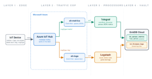
One Device Stream, Two Pipelines: Routing IoT Metrics and Logs into GridDB Cloud with Azure IoT Hub, Telegraf, and Logstash
More
IoT devices can be messy and unweildy. The same sensor that reports a clean temperature reading one second will spit out an ugly, text-based firmware error the next, with both arriving in the same stream. If you force a single tool to handle that mixed data input, you end up compromising somewhere: metrics agents are miserable at parsing free-form text, and log processors are wasteful for high-volume numeric data. In this article we will not compromise. We will build a pipeline that splits the stream at the front door and hands each half to the tool that is good at it: Telegraf, InfluxData’s metrics agent, consumes the clean JSON metrics. Logstash, Elastic’s log processor, uses its grok filters to chop the unstructured firmware errors into queryable fields. Azure IoT Hub sits in front of both, acting as the router that routes each message to the right lane. GridDB Cloud is the destination for everything, using the official Telegraf and Logstash output plugins from the GridDB Cloud v3.2 bundled third-party plugin pack. If you read our previous article on storing OpenTelemetry signals in GridDB Cloud with Kafka, this architecture will feel familiar: a producer at the edge, a routing/buffering layer in the middle, specialized processors, and GridDB Cloud as the vault at the end. The difference is that this time there is zero custom code. Where the Kafka pipeline needed a hand-written Go bridge to flatten OTLP payloads, every stage here is an off-the-shelf component wired together with configuration. Though this blog uses the GridDB Web API, let’s not forget about this recent release: GridDB Cloud v3.2’s non-WebAPI connection support. If you have not read about that release yet, start here: Connecting to GridDB Cloud v3.2 from Your Local Dev Environment. The Architecture: Four Layers The architecture for this is a bit strange; it’s been separated into four parts: Layer 1 — Full data stream of mixed data (edge). Devices emit both signal types into one stream: structured JSON metrics and unstructured text logs, interleaved. Each message carries a small label (msgType) declaring which kind it is. Layer 2 — The router (Azure IoT Hub). IoT Hub’s message routing reads the label and splits the stream: metrics go to one Azure Event Hub, logs go to another. After this point the data is perfectly separated into two independent queues. Layer 3 — The specialized processors (Telegraf and Logstash). Because the split already happened, neither tool has to do a job it is bad at. Telegraf pulls from the metrics queue and parses JSON. Logstash pulls from the logs queue (text) and runs grok. Layer 4 — Datastore (GridDB Cloud). Both tools have an official GridDB output plugin. Telegraf writes its numbers into an optimized TIME_SERIES container; Logstash writes its parsed log rows into its own container. One database, two purpose-built containers. ┌─(msgType='metric')─► Event Hub eh-metrics ─► Telegraf ─► iot_sensor_metrics ┐ device ──► Azure IoT Hub ─┤ ├─ GridDB Cloud └─(msgType='log')────► Event Hub eh-logs ────► Logstash ─► iot_firmware_logs ┘ The two Event Hubs in the middle are queues. The Azure IoT Hub pushes into them; Telegraf and Logstash pull from them at their own pace. That decoupling is what makes the pipeline resilient: if Logstash goes down for an hour, log messages simply pile up in eh-logs and get drained when it comes back. Nothing is lost and nothing blocks the devices. Setting Up the Azure Side We will keep this section brief since the Azure resources are standard. You need: A resource group to hold everything. An Event Hubs namespace (Basic tier is fine — both consumers speak AMQP natively, so you do not need the Kafka-compatible endpoint that Standard tier adds) containing two event hubs: eh-metrics and eh-logs. Two authorization rules per event hub: one with Send rights (used by IoT Hub’s routing endpoints) and one with Listen rights (used by Telegraf and Logstash). Keeping them separate is necessary because mixing them up produces a very specific error. An IoT Hub on the B1 tier or above. The free F1 tier allows only one custom routing endpoint, and this architecture needs two. IoT Hub names are also globally unique across Azure, so pick something distinctive. Two custom endpoints on the IoT Hub, each pointing at one event hub via its Send connection string. Two message routes, which are the heart of the whole design: $ az iot hub message-route create -g <resource-group> -n <iot-hub-name> \ $ –route-name metrics-route –endpoint-name ep-metrics –source devicemessages \ $ –condition "msgType = 'metric'" $ az iot hub message-route create -g <resource-group> -n <iot-hub-name> \ $ –route-name logs-route –endpoint-name ep-logs –source devicemessages \ $ –condition "msgType = 'log'" A device identity for the simulator to authenticate as. Let’s discuss a couple of issues up front: first, IoT Hub routing cannot inspect an arbitrary message body to decide “is this JSON or plain text” — body-based routing queries only work when the message declares contentType = application/json and contentEncoding = utf-8, and plain-text bodies are opaque to the routing engine entirely. The robust pattern is what we use here: the device stamps an application property (msgType) on every message and the routes filter on that property. Second, once you add custom routes, IoT Hub’s fallback route to the built-in endpoint is disabled by default — any message that matches no route is dropped, so a typo in the property name fails silently. Third, on recent Azure CLI versions, creating an event hub on Basic tier requires passing –cleanup-policy Delete –retention-time 24 together (the CLI’s defaults request 7-day retention, which Basic rejects, while the retention flag alone trips a serialization error). Layer 1: The Device Simulator For a data source we will use a small Python script that plays the role of an IoT device. It alternates between two data streams: most of the time it sends a clean JSON metrics payload, and roughly 30% of the time it also emits a raw, syslog-style firmware error line. Crucially, it labels every message with the msgType application property that the routes key on. Install the SDK with pip install azure-iot-device, then: import json, random, time from datetime import datetime, timezone from azure.iot.device import IoTHubDeviceClient, Message CONN = "<your device connection string>" client = IoTHubDeviceClient.create_from_connection_string(CONN) ERRORS = ["E042 sensor read timeout", "E107 fw checksum mismatch", "E019 wifi rssi below threshold"] while True: m = Message(json.dumps({ "deviceId": "sensor-001", "temperature": round(random.uniform(20, 35), 2), "humidity": round(random.uniform(30, 70), 2), })) m.content_type = "application/json" m.content_encoding = "utf-8" m.custom_properties["msgType"] = "metric" client.send_message(m) # occasionally: an ugly text log, labeled for the logs route if random.random() < 0.3: line = f'{datetime.now(timezone.utc).strftime("%Y-%m-%dT%H:%M:%SZ")} sensor-001 ERROR {random.choice(ERRORS)} ip=192.168.1.{random.randint(2,254)}' l = Message(line) l.content_type = "text/plain" l.content_encoding = "utf-8" l.custom_properties["msgType"] = "log" client.send_message(l) time.sleep(3) Get the device connection string with: $ az iot hub device-identity connection-string show -g <resource-group> -n <iot-hub-name> -d sensor-001 -o tsv Before wiring up either consumer, it is worth verifying the split with a throwaway script that reads each event hub directly (the azure-eventhub pip package makes this a ten-liner). You want to see only JSON blobs landing in eh-metrics and only text lines in eh-logs. Debugging the routing and the consumers at the same time is a miserable experience — confirm the iot hub router is doing its job first. Layer 3a: Telegraf — The Metrics Lane Telegraf is InfluxData’s metrics-collection agent. It offers hundreds of input plugins and dozens of output plugins for shipping collected metrics to a time-series store. The GridDB Telegraf plugin is one of those outputs, and conveniently, Telegraf also ships an eventhub_consumer input plugin whose primary use case is exactly this: consuming from Azure Event Hubs and IoT Hub. Building Telegraf With the GridDB Plugin The GridDB output plugin is not distributed as a prebuilt binary, it must be compiled into Telegraf from source. The v3.2 bundled pack ships the plugin source code, which you place into a Telegraf source checkout before building. $ mkdir -p ~/go/src/github.com/influxdata $ cd ~/go/src/github.com/influxdata $ git clone https://github.com/influxdata/telegraf.git $ cd telegraf # Copy in the plugin source from the v3.2 bundle $ cp -r /path/to/telegraf-output-plugin/plugins ./ This places plugins/outputs/griddb/griddb.go into the Telegraf source tree. An important caveat: having the plugin source alone is not sufficient for Telegraf to recognize it. Modern Telegraf (v1.20+) uses a build-tag registration pattern in which each plugin requires a one-line import file under plugins/outputs/all/. Without this file, the plugin compiles into the binary as dead code and Telegraf will reject your configuration with undefined but requested output: griddb. Create plugins/outputs/all/griddb.go: //go:build !custom || outputs || outputs.griddb package all import _ "github.com/influxdata/telegraf/plugins/outputs/griddb" // register plugin Then build and verify: $ make telegraf $ ./telegraf –output-list | grep griddb If griddb appears in the output list, the plugin has been registered correctly. Configuring Telegraf as a Stream Consumer In our previous walkthrough Telegraf played its traditional role of collecting local system metrics. Here it plays a different one: a stream worker that pulls device metrics off an Azure queue. The input section changes; the GridDB output section is identical to before. Create a griddb-iot.conf: $ [[inputs.eventhub_consumer]] $ ## The Listen connection string for eh-metrics, including EntityPath $ connection_string = "Endpoint=sb://<namespace>.servicebus.windows.net/;SharedAccessKeyName=consumer-listen;SharedAccessKey=<key>;EntityPath=eh-metrics" $ data_format = "json" $ json_string_fields = ["deviceId"] $ ## Use the time IoT Hub received the message as the row timestamp $ iot_hub_enqueued_time_as_ts = true $ ## This becomes the GridDB container name $ name_override = "iot_sensor_metrics" $ [[outputs.griddb]] $ api_url = "https://cloud8737.griddb.com:443/griddb/v2/gs_clustermfcloud8737/dbs/nl7QftSt" $ database = "${GRIDDB_DATABASE}" $ cluster_name = "gs_clustermfcloud8737" $ username = "${GRIDDB_USERNAME}" $ password = "${GRIDDB_PASSWORD}" $ update_mode = "append" $ containers = [] $ is_timeseries = true $ timestamp_column = "timestamp" $ [agent] $ interval = "10s" $ flush_interval = "10s" $ metric_batch_size = 1000 $ metric_buffer_limit = 10000 $ omit_hostname = true $ debug = true Adjust the api_url, database, cluster_name, and username values to match your own GridDB Cloud instance, and set is_timeseries = true so the plugin creates a TIME_SERIES container — the appropriate choice for metrics data. Two details worth calling out. omit_hostname = true matters more here than it did before: without it, Telegraf stamps every row with the hostname of the machine running Telegraf, which in an IoT pipeline is misleading — the data came from sensor-001, not from your consumer box, and the deviceId field already carries the real source. And note that eventhub_consumer is a service input: unlike ordinary polling inputs, it listens for events rather than gathering on an interval, which means the –test and –once dry-run flags from our previous walkthrough may produce no output for it. Just run it for real: $ export GRIDDB_PASSWORD='your-password' $ ./telegraf –config griddb-iot.conf With the simulator running, the debug log shows Telegraf writing batches within seconds, and an iot_sensor_metrics container appears in the GridDB Cloud portal with temperature, humidity, and deviceId columns: Layer 3b: Logstash — The Logs Lane Where Telegraf handles metrics, Logstash handles logs. It ingests unstructured text events, parses them into structured fields with its grok filter, and ships them to a destination of your choice. Our destination is GridDB Cloud, and our source is the eh-logs queue full of raw firmware error lines. Installing Logstash The bundle’s README points to a yum-based CentOS install path. On macOS we will download the tarball directly from Elastic — Homebrew’s elastic/tap formula is currently broken on recent Homebrew versions. $ mkdir -p ~/logstash-demo && cd ~/logstash-demo $ curl -O https://artifacts.elastic.co/downloads/logstash/logstash-9.4.1-darwin-aarch64.tar.gz $ tar -xzf logstash-9.4.1-darwin-aarch64.tar.gz $ mv logstash-9.4.1 logstash $ ./logstash/bin/logstash –version Installing the GridDB Output Plugin The plugin ships as a prebuilt .gem, so no Ruby build step is required. Copy it alongside the Logstash install. Note that the leading ./ matters — without it, logstash-plugin treats the argument as a remote plugin name and constructs an invalid URL: $ cp /path/to/logstash-output-plugin/logstash-output-griddb-1.0.0.gem ~/logstash-demo/ $ cd ~/logstash-demo $ ./logstash/bin/logstash-plugin install ./logstash-output-griddb-1.0.0.gem $ ./logstash/bin/logstash-plugin list | grep griddb The input side needs no installation at all: the azure_event_hubs input plugin ships bundled with Logstash. The Logstash Config Save the following as ~/logstash-demo/iot-logs-to-griddb.conf: input { azure_event_hubs { event_hub_connections => ["Endpoint=sb://<namespace>.servicebus.windows.net/;SharedAccessKeyName=consumer-listen;SharedAccessKey=<key>;EntityPath=eh-logs"] initial_position => "beginning" } } filter { grok { match => { "message" => '%{TIMESTAMP_ISO8601:log_ts} %{NOTSPACE:device_id} %{LOGLEVEL:level} %{NOTSPACE:error_code} %{DATA:error_msg} ip=%{IP:device_ip}' } } date { match => [ "log_ts", "ISO8601" ] target => "@timestamp" } mutate { remove_field => [ "message", "log_ts", "event", "log", "@version", "host" ] } } output { stdout { codec => rubydebug } griddb { host => "https://cloud8737.griddb.com:443" cluster => "your-cluster" database => "your-database" container => "iot_firmware_logs" username => "your-username" password => "${GRIDDB_PASSWORD}" insert_mode => "append" } } The grok filter does the core work: it takes a raw line like 2026-07-16T23:28:33Z sensor-001 ERROR E107 fw checksum mismatch ip=192.168.1.99 and breaks it into device_id, level, error_code, error_msg, and device_ip fields. The date filter takes the timestamp embedded inside the log line — the moment the device actually recorded the error — and uses it as the event’s real timestamp, rather than the moment Logstash happened to process it. The connection string deserves special attention, because it bit us twice while building this. It must be the complete string — starting with Endpoint=sb:// and ending with EntityPath=eh-logs — or the plugin fails at startup with Error parsing event hub string name for connection. And it must use the Listen authorization rule, not the Send rule you gave to IoT Hub’s routing endpoints. If you paste the Send string, Logstash connects successfully, discovers the partitions, and then fails on every receive with Unauthorized access. ‘Listen’ claim(s) are required — an error that is easy to miss in the AMQP log spam. You will also see a startup warning that no storage_connection_string is configured. Logstash uses an Azure Storage account to checkpoint its position across restarts and to coordinate multiple Logstash instances; for a single-instance demo it is safe to ignore, at the cost of re-reading the queue from the beginning on each restart. Running It $ cd ~/logstash-demo $ export GRIDDB_PASSWORD='your-password' $ ./logstash/bin/logstash -f iot-logs-to-griddb.conf Startup takes 20–30 seconds. Because of initial_position => “beginning”, Logstash immediately drains everything sitting in eh-logs, so you should see a burst of parsed events scroll past in the rubydebug output, then a steady trickle as the simulator keeps emitting. Each one becomes a row in the iot_firmware_logs container: The resulting schema is clean: one self-documenting column per parsed field, and timestamps that reflect when each error actually occurred on the device. What Lands in GridDB Cloud At this point the full pipeline is live. Two containers, each shaped by the tool that filled it: iot_sensor_metrics — a TIME_SERIES container with one row per metrics message: timestamp, deviceId, temperature, humidity. Created and populated by Telegraf. iot_firmware_logs — one row per parsed firmware error: timestamp, device_id, level, error_code, error_msg, device_ip. Created and populated by Logstash. The same device produced both, the same IoT Hub received both, and the same database stores both — but each signal traveled its own lane and was processed by the tool built for it. A note on topology: in this walkthrough, one machine plays every role — it runs the simulator, Telegraf, and Logstash, so the data flows out to Azure and right back. That looks redundant locally, but it is actually the proof that the architecture is decoupled: no component knows where the others run, because they only ever talk to Azure endpoints. In production, the simulator becomes a fleet of real devices in the field (each with its own IoT Hub device identity), and Telegraf and Logstash become small VMs or containers colocated in the same Azure region as the Event Hubs namespace. Everything in between stays exactly the same. Extra: Grafana Dashboards Over GridDB Cloud The pipeline above is complete on its own, but if you want to visualize what you just ingested, GridDB also ships a Grafana data source plugin in the v3.2 bundle. The installation is somewhat involved, so we are including it here. Important: this plugin is built on AngularJS, which Grafana deprecated in v11 and fully removed in v12. There is no flag or workaround on modern Grafana, as the framework is no longer present. For now, you need Grafana 10.x. You can read more in Grafana’s removal announcement. Installing Grafana 10 Download the last 10.x release directly from Grafana’s download page: $ mkdir -p ~/grafana-demo && cd ~/grafana-demo $ curl -O https://dl.grafana.com/oss/release/grafana-10.4.15.darwin-arm64.tar.gz $ tar -xzf grafana-10.4.15.darwin-arm64.tar.gz $ mv grafana-v10.4.15 grafana Enabling the Plugin Two configuration changes are needed before the plugin will load. Create ~/grafana-demo/grafana/conf/custom.ini (Grafana automatically merges this with the defaults): [plugins] allow_loading_unsigned_plugins = griddb-datasource [security] angular_support_enabled = true The first setting whitelists the unsigned plugin; the second enables the AngularJS compatibility mode that Grafana 10 still provides. Copy the plugin into Grafana’s plugins directory: $ mkdir -p ~/grafana-demo/grafana/data/plugins/griddb-datasource $ cp -r /path/to/grafana-input-plugin/dist/* \ $ ~/grafana-demo/grafana/data/plugins/griddb-datasource/ Start Grafana: $ cd ~/grafana-demo/grafana $ ./bin/grafana server Open http://localhost:3000, log in (admin/admin by default; you will be prompted to set a new password), and add a new GridDB data source under Connections → Data sources. Fill in: Host: https://cloud8737.griddb.com:443 (no trailing path — the plugin appends /griddb/v2/… itself) Cluster: your cluster name Database: your database name User / Password: your GridDB Cloud credentials A Note on the Password Field Once the form is complete, click Save & Test. If the test fails with a TXN_AUTH_FAILED error even though your credentials are correct, the data source form may not have persisted the password to Grafana’s secure storage (this occurred consistently in our testing). You can confirm by inspecting Grafana’s sqlite store: $ sqlite3 ~/grafana-demo/grafana/data/grafana.db \ $ "SELECT name, basic_auth_user, length(secure_json_data) FROM data_source;" If length(secure_json_data) is 2, the password did not save ({} is two characters). The workaround is to set the password via Grafana’s HTTP API, which writes the credentials properly: $ curl -X PUT \ $ -u 'admin:YOUR_GRAFANA_ADMIN_PASSWORD' \ $ -H "Content-Type: application/json" \ $ http://localhost:3000/api/datasources/1 \ $ -d '{ $ "id": 1, $ "name": "griddb-datasource", $ "type": "griddb-datasource", $ "url": "https://cloud8737.griddb.com:443", $ "access": "proxy", $ "basicAuth": true, $ "basicAuthUser": "your-griddb-username", $ "secureJsonData": { "basicAuthPassword": "your-griddb-password" }, $ "jsonData": { $ "xgridcluster": "your-cluster-name", $ "xgriddatabase": "your-database-name", $ "minInterval": "1s" $ } $ }' (Single-quote the -u argument if your Grafana admin password contains shell metacharacters.) After that, secure_json_data will contain a long encrypted blob, and the data source will authenticate cleanly. Querying Your Data With the data source connected, build a panel using the plugin’s query syntax against the containers this pipeline created: $griddb_query_data(iot_sensor_metrics, temperature, select * order by timestamp) The three arguments are the container, the columns to select, and a TQL clause. You can also use $griddb_container_list to populate template variables for a container picker, or $griddb_column_list({container}) to drive column dropdowns. Wrapping Up Four layers, each doing one job: The edge produces a mixed stream of metrics and logs, each message labeled with what it is. Azure IoT Hub routes on that label, splitting the firehose into two clean queues. Telegraf and Logstash each consume the lane they are built for — JSON parsing on one side, grok on the other. GridDB Cloud stores both signals in purpose-built containers, side by side and queryable together. Compared to our Kafka-based OpenTelemetry pipeline, the striking thing about this one is what is missing: there is no bridge, no custom flattening code, no bespoke glue. IoT Hub’s routing rules replace the splitting logic, and the official eventhub_consumer and azure_event_hubs input plugins replace the consuming logic. The GridDB Cloud v3.2 bundled plugin pack supplies both output plugins — one download, and every stage of a cross-cloud IoT pipeline is configuration rather than