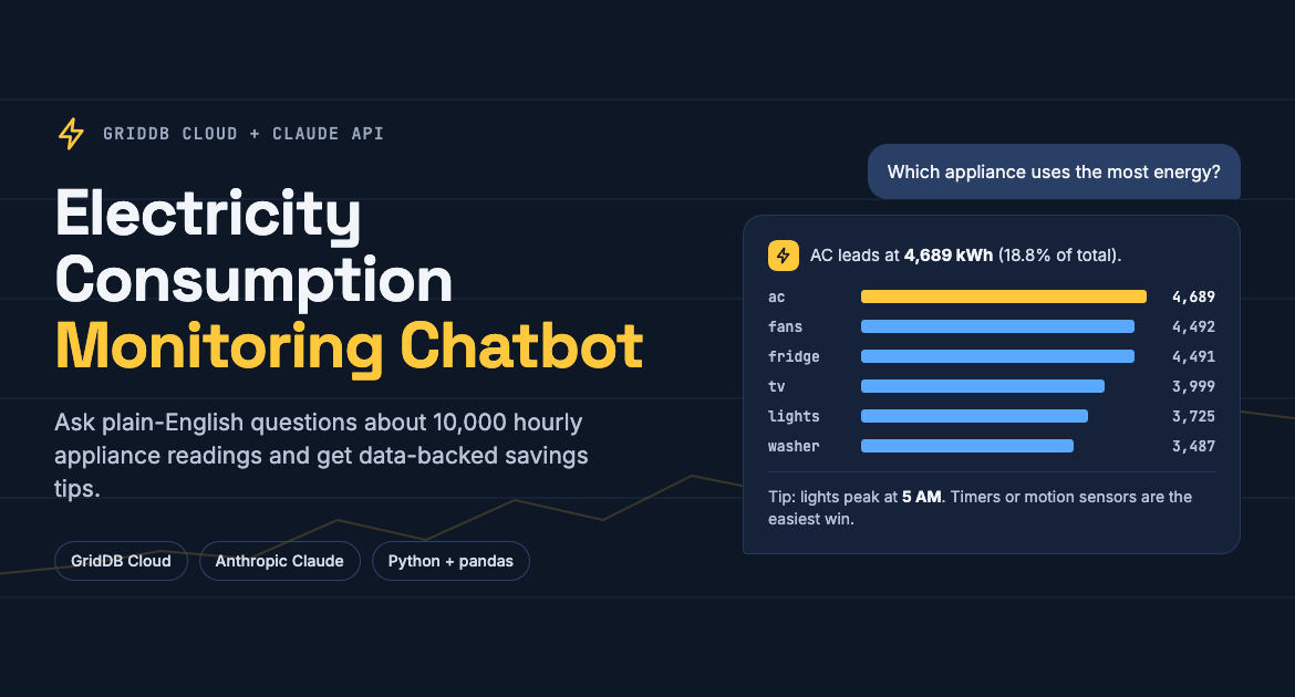
Monitoring household electricity consumption is essential for identifying wasteful patterns and reducing energy costs. However, manually analyzing thousands of hourly readings across multiple appliances is impractical. Combining AI-powered analysis with a high-performance database like GridDB allows you to store, retrieve, and analyze electricity data using natural language queries.
In this article, you will see how to build an AI-powered electricity consumption chatbot using the Anthropic Claude API and GridDB Cloud. The chatbot analyzes 10,000 hourly appliance-level readings, identifies consumption trends, pinpoints peak and off-peak hours for each appliance, and provides data-backed recommendations to save electricity. We will also use AI to create data visualizations showing electricity consumption trends.
Note: We have the full jupyter notebook output of this blog below article text.
GridDB’s efficient handling of time-series data, combined with Claude’s analytical reasoning, provides a powerful way to turn raw electricity readings into actionable insights.
Prerequisites:
You will need the following to run scripts in this article:
- A GridDB cloud account. Refer to this quick start guide to set up a GridDB cloud account.
- Anthropic API Key. You can obtain one from the Anthropic console.
Note: You can find the complete code for this tutorial in my GridDB Blogs GitHub repository.
Installing and Importing Required Libraries
The following installs the libraries you will need to run the scripts in this article.
!pip install python-dotenv
!pip install anthropic
The script below imports the required libraries.
import pandas as pd
import matplotlib.pyplot as plt
import base64
import os
import requests
import json
import re

from dotenv import load_dotenv
load_dotenv()
Importing the Dataset
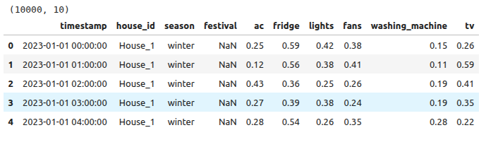
The dataset used in this article provides hourly electricity consumption data recorded at the appliance level. It includes readings for six appliances: air conditioner (ac), fridge, lights, fans, washing machine, and TV. Each row represents one hourly reading for a household, along with metadata such as the season and any ongoing festival. You can download the dataset from Kaggle.
The following script loads the dataset and selects the first 10,000 records. The original dataset contains more than 400k records; however, 10k records are sufficient for this sample analysis.
dataset = pd.read_csv("appliance_usage_dataset.csv",
                      encoding = 'utf-8')
dataset = dataset[:10000]
print(dataset.shape)
dataset.head()
Output:
Inserting Data in GridDB
We will insert the data into GridDB Cloud.
Creating a GridDB Connection
Run the following script to test your connection with the GridDB cloud. You can retrieve the connection credentials from your GridDB cloud account.
username = os.environ.get("username")
password = os.environ.get("password")
base_url = os.environ.get("base_url")


url = f"{base_url}/checkConnection"

credentials = f"{username}:{password}"
encoded_credentials = base64.b64encode(credentials.encode()).decode()

headers = {
    'Content-Type': 'application/json',  # Added this header to specify JSON content
    'Authorization': f'Basic {encoded_credentials}',
    'User-Agent': 'PostmanRuntime/7.29.0'
}

response = requests.get(url, headers=headers)

print(response.status_code)
Output:
200If you do not see the above response, check this quick start guide for troubleshooting.
Creating a GridDB Container for Electricity Consumption Data
Before inserting data, we need to create a container in GridDB with the correct schema. The following script maps pandas data types to GridDB types.
dataset.insert(0, "SerialNo", dataset.index + 1)
dataset.columns.name = None
# Mapping pandas dtypes to GridDB types
type_mapping = {
    "int64":          "LONG",
    "float64":        "DOUBLE",
    "bool":           "BOOL",
    'datetime64': "TIMESTAMP",
    "object":         "STRING",
    "category":       "STRING",
}

# Generate the columns part of the payload dynamically
columns = []
for col, dtype in dataset.dtypes.items():
    griddb_type = type_mapping.get(str(dtype), "STRING")  # Default to STRING if unknown
    columns.append({
        "name": col,
        "type": griddb_type
    })

print(columns)
Output:

Next, we create the container using the GridDB REST API.
container_name = "electricity_consumption_db"

url = f"{base_url}/containers"

# Create the payload for the POST request
payload = json.dumps({
    "container_name": container_name,
    "container_type": "COLLECTION",
    "rowkey": True,  # Assuming the first column as rowkey
    "columns": columns
})


# Make the POST request to create the container
response = requests.post(url, headers=headers, data=payload)

# Print the response
print(f"Status Code: {response.status_code}")
Output:
Status Code: 201The 201 status code confirms the container has been created successfully.
Inserting Data in Electricity Consumption GridDB Container
With the container created, we can now insert the 10,000 rows of electricity consumption data. The format_row function handles type conversions, including converting NaN values to None for GridDB compatibility.
url = f"{base_url}/containers/{container_name}/rows"
# Convert dataset to list of lists (row-wise) with proper formatting

def format_row(row):
    formatted = []
    for item in row:
        if pd.isna(item):
            formatted.append(None)  # Convert NaN to None
        elif isinstance(item, bool):
            formatted.append(str(item).lower())  # Convert True/False to true/false
        elif isinstance(item, (int, float)):
            formatted.append(item)  # Keep integers and floats as they are
        else:
            formatted.append(str(item))  # Convert other types to string
    return formatted

# Prepare rows with correct formatting
rows = [format_row(row) for row in dataset.values.tolist()]

# Create payload as a JSON string
payload = json.dumps(rows)

# Make the PUT request to add the rows to the container
response = requests.put(url, headers=headers, data=payload)

# Print the response
print(f"Status Code: {response.status_code}")
print(f"Response Text: {response.text}")
Output:
Status Code: 200
Response Text: {"count":10000}
At this point, all 10,000 records have been successfully inserted into the GridDB container.
Using AI to Monitor Electricity Consumption and Get Recommendations
Now that the data is stored in GridDB, we can retrieve it and use the Anthropic Claude API to analyze consumption patterns and provide recommendations. The approach involves three steps: retrieve data from GridDB, build a pre-computed summary of the dataset, and pass that summary to Claude as context for intelligent Q&A.
Retrieve Data from GridDB
The following script retrieves all 10,000 records from the GridDB container and loads them into a pandas DataFrame.
url = f"{base_url}/containers/{container_name}/rows"

# Define the payload for the query
payload = json.dumps({
    "offset": 0,           # Start from the first row
    "limit": 10000,         # Limit the number of rows returned
    "condition": "",       # No filtering condition (you can customize it)
    "sort": ""             # No sorting (you can customize it)
})

# Make the POST request to read data from the container
response = requests.post(url, headers=headers, data=payload)

# Check response status and print output
print(f"Status Code: {response.status_code}")
if response.status_code == 200:
    try:
        data = response.json()
        print("Data retrieved successfully!")

        # Convert the response to a DataFrame
        rows = data.get("rows", [])
        electricity_consumption_db = pd.DataFrame(rows, columns=[col for col in dataset.columns])

    except json.JSONDecodeError:
        print("Error: Failed to decode JSON response.")
else:
    print(f"Error: Failed to query data from the container. Response: {response.text}")

print(electricity_consumption_db.shape)
electricity_consumption_db.head()
Output:
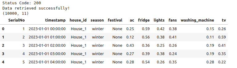
The data has been successfully retrieved from GridDB and is ready for analysis.
Build Dataset Summary
Since we cannot send 10,000 raw rows to Claude in a single prompt because it may exceed token limits and reduce response quality, we pre-compute comprehensive aggregations and pass those as context instead. This way, Claude reasons over actual statistics computed from all 10,000 records.
import pandas as pd

APPLIANCE_COLS = ['ac', 'fridge', 'lights', 'fans', 'washing_machine', 'tv']

# Prepare the dataframe
electricity_consumption_db['timestamp'] = pd.to_datetime(electricity_consumption_db['timestamp'])
electricity_consumption_db['Hour'] = electricity_consumption_db['timestamp'].dt.hour
electricity_consumption_db['DayOfWeek'] = electricity_consumption_db['timestamp'].dt.day_name()
electricity_consumption_db['Month'] = electricity_consumption_db['timestamp'].dt.month
electricity_consumption_db['total_kwh'] = electricity_consumption_db[APPLIANCE_COLS].sum(axis=1)


def build_summary(df):
    parts = []

    # Overview
    parts.append(f"Records: {len(df)} hourly readings across {df['house_id'].nunique()} households")
    parts.append(f"Period: {df['timestamp'].min()} to {df['timestamp'].max()}")
    parts.append(f"Seasons: {df['season'].unique().tolist()}")
    parts.append(f"Festivals: {df['festival'].unique().tolist()}")

    # Appliance stats
    parts.append(f"\n--- Appliance Stats (kWh) ---\n{df[APPLIANCE_COLS].describe().round(3).to_string()}")

    # Total energy ranking
    totals = df[APPLIANCE_COLS].sum().sort_values(ascending=False)
    pct = (totals / totals.sum() * 100).round(1)
    parts.append(f"\n--- Energy Ranking ---")
    for app in totals.index:
        parts.append(f"  {app}: {totals[app]:.1f} kWh ({pct[app]}%)")

    # Hourly patterns
    hourly = df.groupby('Hour')[APPLIANCE_COLS].mean().round(4)
    hourly_total = df.groupby('Hour')['total_kwh'].mean().round(2)
    parts.append(f"\n--- Hourly Avg Consumption (kWh) ---\n{hourly.to_string()}")
    parts.append(f"\nHourly total avg:\n{hourly_total.to_string()}")
    parts.append(f"Lowest hour: {hourly_total.idxmin()}:00 ({hourly_total.min()} kWh)")
    parts.append(f"Highest hour: {hourly_total.idxmax()}:00 ({hourly_total.max()} kWh)")

    # Peak per appliance
    parts.append(f"\n--- Peak/Low Hour per Appliance ---")
    for col in APPLIANCE_COLS:
        parts.append(f"  {col}: peak {hourly[col].idxmax()}:00 ({hourly[col].max()}), low {hourly[col].idxmin()}:00 ({hourly[col].min()})")

    # Season patterns
    seasonal = df.groupby('season')[APPLIANCE_COLS].mean().round(4)
    parts.append(f"\n--- Seasonal Avg (kWh) ---\n{seasonal.to_string()}")

    # Day of week
    day_order = ['Monday', 'Tuesday', 'Wednesday', 'Thursday', 'Friday', 'Saturday', 'Sunday']
    daily = df.groupby('DayOfWeek')['total_kwh'].mean().reindex(day_order).round(2)
    parts.append(f"\n--- Day of Week Avg Total (kWh) ---\n{daily.to_string()}")

    # Household comparison (top 5 and bottom 5)
    hh = df.groupby('house_id')['total_kwh'].mean().sort_values(ascending=False).round(2)
    parts.append(f"\n--- Household Avg Hourly (kWh) ---")
    parts.append(f"Top 5:\n{hh.head().to_string()}")
    parts.append(f"Bottom 5:\n{hh.tail().to_string()}")

    # Festival impact
    fest = df.groupby('festival')['total_kwh'].mean().round(2)
    parts.append(f"\n--- Festival Impact (avg kWh) ---\n{fest.to_string()}")

    return "\n".join(parts)


data_summary = build_summary(electricity_consumption_db)
The build_summary function in the above script computes seven categories of aggregations: overall statistics, appliance energy rankings with percentage shares, hourly consumption patterns with peak and off-peak hours for each appliance, seasonal averages, day-of-week trends, household comparisons, and festival impact analysis. These aggregations cover all 10,000 records and give Claude a comprehensive view of the data.
Create Chatbot
With the data summary ready, we create the chatbot. The system prompt embeds the entire summary and instructs Claude to always cite specific numbers from the data. The ElectricityChatbot class maintains conversation history, allowing follow-up questions that build on previous answers.
In the script below, We used the Claude 4.6 sonnet model for reasoning. You can use any other anthropic model if you want.
SYSTEM_PROMPT = f"""You are an electricity consumption analyst. You have data from {electricity_consumption_db['house_id'].nunique()} households
with {len(electricity_consumption_db)} hourly readings. Appliance columns: ac, fridge, lights, fans, washing_machine, tv.
All values are in kWh. The data also has season and festival columns.

Always cite specific numbers. Estimate kWh savings when giving recommendations.

DATA:
{data_summary}
"""


class ElectricityChatbot:
    def __init__(self):
        self.client = anthropic.Anthropic()
        self.history = []

    def ask(self, question):
        self.history.append({"role": "user", "content": question})
        response = self.client.messages.create(
            model="claude-sonnet-4-6",
            max_tokens=2048,
            system=SYSTEM_PROMPT,
            messages=self.history
        )
        answer = response.content[0].text
        self.history.append({"role": "assistant", "content": answer})
        return answer

    def reset(self):
        self.history = []
        print("History cleared.")


chatbot = ElectricityChatbot()
print("Chatbot ready!")
Output:
Chatbot ready!The chatbot is initialized and ready to answer questions about the electricity data.
Ask Questions
Let’s test the chatbot with questions about electricity consumption trends, savings recommendations, and targeted advice.
Question 1: Electricity Consumption Trends
print(chatbot.ask("What are the main electricity consumption trends? Break down by appliance and season."))Output (partial screenshot):
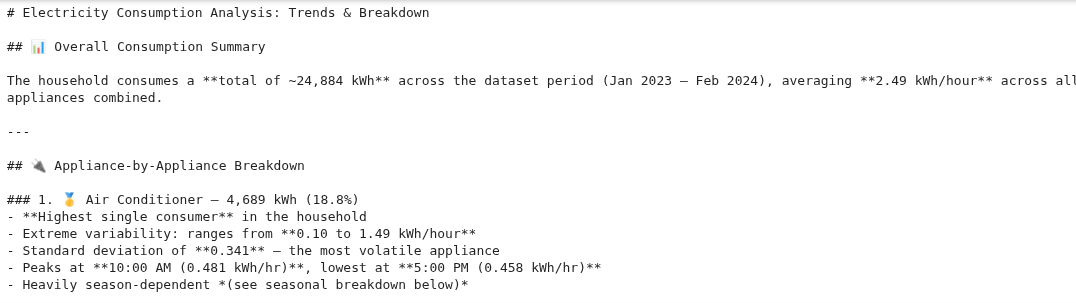
The chatbot provides a detailed breakdown of consumption patterns. It identifies the air conditioner as the highest single consumer at 4,689 kWh (18.8% of total), followed closely by fans at 4,492 kWh (18.1%) and fridge at 4,491 kWh (18.0%). The analysis reveals striking seasonal patterns: AC consumption jumps to 1.058 kWh/hr in summer (a 3.5x increase over winter), while fans and washing machines surge dramatically during the rainy season. The fridge and TV remain remarkably stable across all seasons, making them low-priority targets for optimization.
Question 2: Savings Recommendations
print(chatbot.ask("Give me specific recommendations to save electricity with estimated kWh savings for each."))Output (partial screenshot):
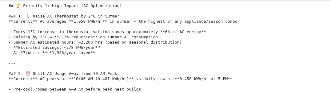
Claude provides prioritized recommendations with estimated kWh savings based on the actual data. The top recommendations include: raising the AC thermostat by 2°C in summer (saving approximately 278 kWh/year), setting AC auto-shutoff during winter nights (saving approximately 383 kWh/year), replacing non-LED lights (saving approximately 670 kWh/year), and addressing the unusual 5 AM lighting peak which suggests lights being left on overnight (saving approximately 420 kWh/year). Each recommendation includes the specific data points that support it.
Question 3: Best Single Change
print(chatbot.ask("Which single change gives the biggest savings with least effort?"))Output (partial screenshot):
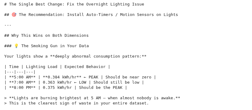
Because the chatbot maintains conversation history, this follow-up question builds on the previous analysis. Claude identifies the overnight lighting issue as the single best change: the data shows lights peaking at 5 AM (0.384 kWh/hr) when they should be near zero, suggesting lights are left on overnight.
Execute Code and Generate Charts
In addition to natural language analysis, we can ask Claude to generate matplotlib code for visualizations. The generate_and_run_chart function sends a chart description to Claude, receives executable Python code, and runs it inline to display the chart.
def generate_and_run_chart(question):
    """
    Ask Claude to generate matplotlib code for a chart, then execute it.
    The chart displays inline in the notebook.
    """
    schema = f"Columns: {list(electricity_consumption_db.columns)}\nAppliance cols: {APPLIANCE_COLS}\nSample:\n{electricity_consumption_db.head(3).to_csv(index=False)}"

    response = client.messages.create(
        model="claude-sonnet-4-6",
        max_tokens=2048,
        messages=[{
            "role": "user",
            "content": f"""I have a pandas DataFrame `electricity_consumption_db` with this structure:

{schema}

The electricity_consumption_db already has 'Hour', 'DayOfWeek', 'Month', 'total_kwh' columns.
Appliance values (ac, fridge, lights, fans, washing_machine, tv) are in kWh.

Write Python code using pandas and matplotlib to: {question}

RULES:
- Return ONLY Python code, no markdown fences, no explanation
- df is already loaded, matplotlib.pyplot is imported as plt
- Use plt.figure(figsize=(10, 6)) for good sizing
- Always include plt.tight_layout() and plt.show()
- Add clear title, axis labels, and legend where needed"""
        }]
    )

    code = response.content[0].text
    # Strip markdown fences if Claude includes them
    code = re.sub(r'^
python\s*’, ”, code, flags=re.MULTILINE)
code = re.sub(r’^\s*$', '', code, flags=re.MULTILINE)
code = code.strip()
print("Generated code:")
print("-" * 40)
print(code)
print("-" * 40)
print("\nExecuting...\n")
exec(code, globals())
The `generate_and_run_chart` function sends the dataframe schema and a natural language description to Claude, which returns ready-to-execute matplotlib code. The `exec(code, globals())` call runs the code in the global scope so that all variables (including electricity_consumption_db, plt, and pd) are accessible.
Let's plot some charts showing electricity consumption trends.

#### Chart 1: Hourly Consumption by Appliance
python
generate_and_run_chart("Line chart showing average hourly consumption for each appliance, all on one plot with different colors and a legend.")
**Output:**

<img src="images\img7-average-hourly-consumption-by-appliance.png">


#### Chart 2: Total Energy by Appliance
python
generate_and_run_chart("Bar chart showing total energy consumption per appliance, sorted highest to lowest, with kWh values on each bar.")
**Output:**

<img src="images\img8-total-energy-consumptio-per-appliance.png">

The bar chart confirms AC as the highest total consumer at 4,689 kWh, followed by fans and fridge, with washing machine consuming the least at 3,487 kWh.

#### Chart 3: Seasonal Patterns
python
generate_and_run_chart("Bar chart showing daily average consumption of each device for all the seasons")
Output:
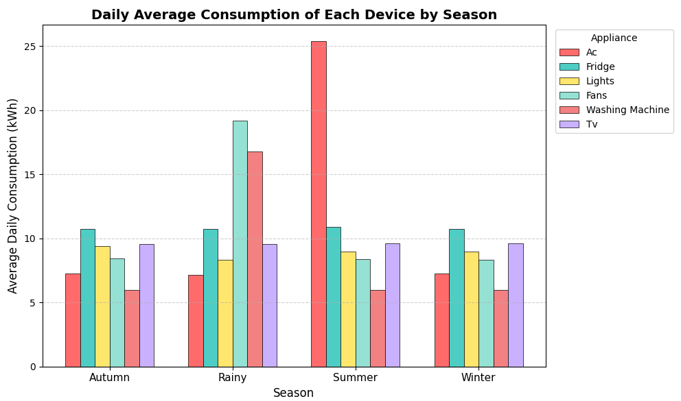
The seasonal chart highlights the dramatic AC spike in summer and the fan and washing machine surges during the rainy season, while fridge and TV remain stable across all seasons.
Conclusion
This article demonstrates how to use the Anthropic Claude API and GridDB Cloud to build an AI-powered electricity consumption chatbot, which delivers data-backed analysis of consumption trends, identifies peak and off-peak hours for each appliance, and provides actionable savings recommendations with estimated kWh reductions. The code generation capability extends the chatbot further by producing inline matplotlib visualizations on demand, making it easy to explore the data visually without writing chart code manually.
You can extend this approach by adding more households for comparative analysis, integrating real-time data feeds from smart meters, or combining the chatbot with GridDB’s time-series querying capabilities for more granular analysis. The combination of a high-performance database and AI reasoning opens up possibilities for intelligent energy monitoring at scale.
You can find the complete code for this blog on the GridDB Blogs GitHub repository. If you have any questions or queries related to GridDB, create a post on Stack Overflow with the griddb tag. Our engineers are more than happy to respond.
Jupyter Notebook Output
Installing and Importing Required Libraries
!pip install python-dotenv
!pip install anthropic
Defaulting to user installation because normal site-packages is not writeable
Requirement already satisfied: python-dotenv in /home/mani/.local/lib/python3.10/site-packages (1.2.1)

[notice] A new release of pip is available: 25.3 -> 26.0.1
[notice] To update, run: python3 -m pip install --upgrade pip
Defaulting to user installation because normal site-packages is not writeable
Collecting anthropic
  Downloading anthropic-0.84.0-py3-none-any.whl.metadata (3.0 kB)
Requirement already satisfied: anyio<5,>=3.5.0 in /home/mani/.local/lib/python3.10/site-packages (from anthropic) (4.3.0)
Requirement already satisfied: distro<2,>=1.7.0 in /usr/lib/python3/dist-packages (from anthropic) (1.7.0)
Collecting docstring-parser<1,>=0.15 (from anthropic)
  Using cached docstring_parser-0.17.0-py3-none-any.whl.metadata (3.5 kB)
Requirement already satisfied: httpx<1,>=0.25.0 in /home/mani/.local/lib/python3.10/site-packages (from anthropic) (0.28.1)
Requirement already satisfied: jiter<1,>=0.4.0 in /home/mani/.local/lib/python3.10/site-packages (from anthropic) (0.7.0)
Requirement already satisfied: pydantic<3,>=1.9.0 in /home/mani/.local/lib/python3.10/site-packages (from anthropic) (2.11.7)
Requirement already satisfied: sniffio in /home/mani/.local/lib/python3.10/site-packages (from anthropic) (1.3.1)
Requirement already satisfied: typing-extensions<5,>=4.10 in /home/mani/.local/lib/python3.10/site-packages (from anthropic) (4.15.0)
Requirement already satisfied: idna>=2.8 in /usr/lib/python3/dist-packages (from anyio<5,>=3.5.0->anthropic) (3.3)
Requirement already satisfied: exceptiongroup>=1.0.2 in /home/mani/.local/lib/python3.10/site-packages (from anyio<5,>=3.5.0->anthropic) (1.3.0)
Requirement already satisfied: certifi in /home/mani/.local/lib/python3.10/site-packages (from httpx<1,>=0.25.0->anthropic) (2025.10.5)
Requirement already satisfied: httpcore==1.* in /home/mani/.local/lib/python3.10/site-packages (from httpx<1,>=0.25.0->anthropic) (1.0.4)
Requirement already satisfied: h11<0.15,>=0.13 in /home/mani/.local/lib/python3.10/site-packages (from httpcore==1.*->httpx<1,>=0.25.0->anthropic) (0.14.0)
Requirement already satisfied: annotated-types>=0.6.0 in /home/mani/.local/lib/python3.10/site-packages (from pydantic<3,>=1.9.0->anthropic) (0.7.0)
Requirement already satisfied: pydantic-core==2.33.2 in /home/mani/.local/lib/python3.10/site-packages (from pydantic<3,>=1.9.0->anthropic) (2.33.2)
Requirement already satisfied: typing-inspection>=0.4.0 in /home/mani/.local/lib/python3.10/site-packages (from pydantic<3,>=1.9.0->anthropic) (0.4.0)
Downloading anthropic-0.84.0-py3-none-any.whl (455 kB)
Using cached docstring_parser-0.17.0-py3-none-any.whl (36 kB)
Installing collected packages: docstring-parser, anthropic
   ━━━━━━━━━━━━━━━━━━━━━━━━━━━━━━━━━━━━━━━━ 2/2 [anthropic]━ 1/2 [anthropic]
Successfully installed anthropic-0.84.0 docstring-parser-0.17.0

[notice] A new release of pip is available: 25.3 -> 26.0.1
[notice] To update, run: python3 -m pip install --upgrade pip
import pandas as pd
import matplotlib.pyplot as plt
import base64
import os
import requests
import json
import re

from dotenv import load_dotenv
load_dotenv()
True
Importing the Dataset
dataset = pd.read_csv("appliance_usage_dataset.csv",
                      encoding = 'utf-8')
dataset = dataset[:10000]
print(dataset.shape)
dataset.head()
(10000, 10)
| timestamp | house_id | season | festival | ac | fridge | lights | fans | washing_machine | tv | |
|---|---|---|---|---|---|---|---|---|---|---|
| 0 | 2023-01-01 00:00:00 | House_1 | winter | NaN | 0.25 | 0.59 | 0.42 | 0.38 | 0.15 | 0.26 |
| 1 | 2023-01-01 01:00:00 | House_1 | winter | NaN | 0.12 | 0.56 | 0.38 | 0.41 | 0.11 | 0.59 |
| 2 | 2023-01-01 02:00:00 | House_1 | winter | NaN | 0.43 | 0.36 | 0.25 | 0.26 | 0.19 | 0.41 |
| 3 | 2023-01-01 03:00:00 | House_1 | winter | NaN | 0.27 | 0.39 | 0.38 | 0.24 | 0.19 | 0.35 |
| 4 | 2023-01-01 04:00:00 | House_1 | winter | NaN | 0.28 | 0.54 | 0.26 | 0.35 | 0.28 | 0.22 |
Inserting Data in GridDB
Creating a GridDB Connection
username = os.environ.get("username")
password = os.environ.get("password")
base_url = os.environ.get("base_url")


url = f"{base_url}/checkConnection"

credentials = f"{username}:{password}"
encoded_credentials = base64.b64encode(credentials.encode()).decode()

headers = {
    'Content-Type': 'application/json',  # Added this header to specify JSON content
    'Authorization': f'Basic {encoded_credentials}',
    'User-Agent': 'PostmanRuntime/7.29.0'
}

response = requests.get(url, headers=headers)

print(response.status_code)
print(response.text)
200
Creating a GridDB Container for Electricity Consumption Data
dataset.insert(0, "SerialNo", dataset.index + 1)
dataset.columns.name = None
# Mapping pandas dtypes to GridDB types
type_mapping = {
    "int64":          "LONG",
    "float64":        "DOUBLE",
    "bool":           "BOOL",
    'datetime64': "TIMESTAMP",
    "object":         "STRING",
    "category":       "STRING",
}

# Generate the columns part of the payload dynamically
columns = []
for col, dtype in dataset.dtypes.items():
    griddb_type = type_mapping.get(str(dtype), "STRING")  # Default to STRING if unknown
    columns.append({
        "name": col,
        "type": griddb_type
    })

print(columns)
[{'name': 'SerialNo', 'type': 'LONG'}, {'name': 'timestamp', 'type': 'STRING'}, {'name': 'house_id', 'type': 'STRING'}, {'name': 'season', 'type': 'STRING'}, {'name': 'festival', 'type': 'STRING'}, {'name': 'ac', 'type': 'DOUBLE'}, {'name': 'fridge', 'type': 'DOUBLE'}, {'name': 'lights', 'type': 'DOUBLE'}, {'name': 'fans', 'type': 'DOUBLE'}, {'name': 'washing_machine', 'type': 'DOUBLE'}, {'name': 'tv', 'type': 'DOUBLE'}]
container_name = "electricity_consumption_db"

url = f"{base_url}/containers"

# Create the payload for the POST request
payload = json.dumps({
    "container_name": container_name,
    "container_type": "COLLECTION",
    "rowkey": True,  # Assuming the first column as rowkey
    "columns": columns
})


# Make the POST request to create the container
response = requests.post(url, headers=headers, data=payload)

# Print the response
print(f"Status Code: {response.status_code}")
Status Code: 201
Inserting Data in Electricity Consumption GridDB Container
url = f"{base_url}/containers/{container_name}/rows"
# Convert dataset to list of lists (row-wise) with proper formatting

def format_row(row):
    formatted = []
    for item in row:
        if pd.isna(item):
            formatted.append(None)  # Convert NaN to None
        elif isinstance(item, bool):
            formatted.append(str(item).lower())  # Convert True/False to true/false
        elif isinstance(item, (int, float)):
            formatted.append(item)  # Keep integers and floats as they are
        else:
            formatted.append(str(item))  # Convert other types to string
    return formatted

# Prepare rows with correct formatting
rows = [format_row(row) for row in dataset.values.tolist()]

# Create payload as a JSON string
payload = json.dumps(rows)

# Make the PUT request to add the rows to the container
response = requests.put(url, headers=headers, data=payload)

# Print the response
print(f"Status Code: {response.status_code}")
print(f"Response Text: {response.text}")
Status Code: 200
Response Text: {"count":10000}
Using AI to Monitor Electricity Consumption and Get Recommendations
Retrieve Data from GridDB
url = f"{base_url}/containers/{container_name}/rows"

# Define the payload for the query
payload = json.dumps({
    "offset": 0,           # Start from the first row
    "limit": 10000,         # Limit the number of rows returned
    "condition": "",       # No filtering condition (you can customize it)
    "sort": ""             # No sorting (you can customize it)
})

# Make the POST request to read data from the container
response = requests.post(url, headers=headers, data=payload)

# Check response status and print output
print(f"Status Code: {response.status_code}")
if response.status_code == 200:
    try:
        data = response.json()
        print("Data retrieved successfully!")

        # Convert the response to a DataFrame
        rows = data.get("rows", [])
        electricity_consumption_db = pd.DataFrame(rows, columns=[col for col in dataset.columns])

    except json.JSONDecodeError:
        print("Error: Failed to decode JSON response.")
else:
    print(f"Error: Failed to query data from the container. Response: {response.text}")

print(electricity_consumption_db.shape)
electricity_consumption_db.head()
Status Code: 200
Data retrieved successfully!
(10000, 11)
| SerialNo | timestamp | house_id | season | festival | ac | fridge | lights | fans | washing_machine | tv | |
|---|---|---|---|---|---|---|---|---|---|---|---|
| 0 | 1 | 2023-01-01 00:00:00 | House_1 | winter | None | 0.25 | 0.59 | 0.42 | 0.38 | 0.15 | 0.26 |
| 1 | 2 | 2023-01-01 01:00:00 | House_1 | winter | None | 0.12 | 0.56 | 0.38 | 0.41 | 0.11 | 0.59 |
| 2 | 3 | 2023-01-01 02:00:00 | House_1 | winter | None | 0.43 | 0.36 | 0.25 | 0.26 | 0.19 | 0.41 |
| 3 | 4 | 2023-01-01 03:00:00 | House_1 | winter | None | 0.27 | 0.39 | 0.38 | 0.24 | 0.19 | 0.35 |
| 4 | 5 | 2023-01-01 04:00:00 | House_1 | winter | None | 0.28 | 0.54 | 0.26 | 0.35 | 0.28 | 0.22 |
Build Dataset Summary
import pandas as pd

APPLIANCE_COLS = ['ac', 'fridge', 'lights', 'fans', 'washing_machine', 'tv']

# Prepare the dataframe
electricity_consumption_db['timestamp'] = pd.to_datetime(electricity_consumption_db['timestamp'])
electricity_consumption_db['Hour'] = electricity_consumption_db['timestamp'].dt.hour
electricity_consumption_db['DayOfWeek'] = electricity_consumption_db['timestamp'].dt.day_name()
electricity_consumption_db['Month'] = electricity_consumption_db['timestamp'].dt.month
electricity_consumption_db['total_kwh'] = electricity_consumption_db[APPLIANCE_COLS].sum(axis=1)


def build_summary(df):
    parts = []

    # Overview
    parts.append(f"Records: {len(df)} hourly readings across {df['house_id'].nunique()} households")
    parts.append(f"Period: {df['timestamp'].min()} to {df['timestamp'].max()}")
    parts.append(f"Seasons: {df['season'].unique().tolist()}")
    parts.append(f"Festivals: {df['festival'].unique().tolist()}")

    # Appliance stats
    parts.append(f"\n--- Appliance Stats (kWh) ---\n{df[APPLIANCE_COLS].describe().round(3).to_string()}")

    # Total energy ranking
    totals = df[APPLIANCE_COLS].sum().sort_values(ascending=False)
    pct = (totals / totals.sum() * 100).round(1)
    parts.append(f"\n--- Energy Ranking ---")
    for app in totals.index:
        parts.append(f"  {app}: {totals[app]:.1f} kWh ({pct[app]}%)")

    # Hourly patterns
    hourly = df.groupby('Hour')[APPLIANCE_COLS].mean().round(4)
    hourly_total = df.groupby('Hour')['total_kwh'].mean().round(2)
    parts.append(f"\n--- Hourly Avg Consumption (kWh) ---\n{hourly.to_string()}")
    parts.append(f"\nHourly total avg:\n{hourly_total.to_string()}")
    parts.append(f"Lowest hour: {hourly_total.idxmin()}:00 ({hourly_total.min()} kWh)")
    parts.append(f"Highest hour: {hourly_total.idxmax()}:00 ({hourly_total.max()} kWh)")

    # Peak per appliance
    parts.append(f"\n--- Peak/Low Hour per Appliance ---")
    for col in APPLIANCE_COLS:
        parts.append(f"  {col}: peak {hourly[col].idxmax()}:00 ({hourly[col].max()}), low {hourly[col].idxmin()}:00 ({hourly[col].min()})")

    # Season patterns
    seasonal = df.groupby('season')[APPLIANCE_COLS].mean().round(4)
    parts.append(f"\n--- Seasonal Avg (kWh) ---\n{seasonal.to_string()}")

    # Day of week
    day_order = ['Monday', 'Tuesday', 'Wednesday', 'Thursday', 'Friday', 'Saturday', 'Sunday']
    daily = df.groupby('DayOfWeek')['total_kwh'].mean().reindex(day_order).round(2)
    parts.append(f"\n--- Day of Week Avg Total (kWh) ---\n{daily.to_string()}")

    # Household comparison (top 5 and bottom 5)
    hh = df.groupby('house_id')['total_kwh'].mean().sort_values(ascending=False).round(2)
    parts.append(f"\n--- Household Avg Hourly (kWh) ---")
    parts.append(f"Top 5:\n{hh.head().to_string()}")
    parts.append(f"Bottom 5:\n{hh.tail().to_string()}")

    # Festival impact
    fest = df.groupby('festival')['total_kwh'].mean().round(2)
    parts.append(f"\n--- Festival Impact (avg kWh) ---\n{fest.to_string()}")

    return "\n".join(parts)


data_summary = build_summary(electricity_consumption_db)
print(data_summary[:2000])
Records: 10000 hourly readings across 1 households
Period: 2023-01-01 00:00:00 to 2024-02-21 15:00:00
Seasons: ['winter', 'summer', 'rainy', 'autumn']
Festivals: [None, 'makar sankranti', 'mahashivratri', 'holi', 'ram navmi', 'ganesh chaturthi', 'navratri', 'dusshera', 'diwali', 'christmas']

--- Appliance Stats (kWh) ---
              ac     fridge     lights       fans  washing_machine         tv
count  10000.000  10000.000  10000.000  10000.000        10000.000  10000.000
mean       0.469      0.449      0.373      0.449            0.349      0.400
std        0.341      0.087      0.176      0.210            0.210      0.116
min        0.100      0.300      0.200      0.200            0.100      0.200
25%        0.230      0.370      0.280      0.300            0.200      0.300
50%        0.360      0.450      0.350      0.390            0.290      0.400
75%        0.480      0.520      0.430      0.490            0.390      0.500
max        1.490      0.600      1.650      1.090            1.000      0.600

--- Energy Ranking ---
  ac: 4689.3 kWh (18.8%)
  fans: 4492.2 kWh (18.1%)
  fridge: 4491.2 kWh (18.0%)
  tv: 3998.6 kWh (16.1%)
  lights: 3725.5 kWh (15.0%)
  washing_machine: 3487.3 kWh (14.0%)

--- Hourly Avg Consumption (kWh) ---
          ac  fridge  lights    fans  washing_machine      tv
Hour
0     0.4753  0.4503  0.3698  0.4484           0.3434  0.4014
1     0.4693  0.4536  0.3732  0.4485           0.3411  0.3918
2     0.4610  0.4479  0.3714  0.4539           0.3486  0.3988
3     0.4641  0.4518  0.3688  0.4502           0.3423  0.4011
4     0.4626  0.4468  0.3797  0.4478           0.3516  0.3900
5     0.4676  0.4428  0.3837  0.4480           0.3495  0.4023
6     0.4734  0.4408  0.3726  0.4446           0.3489  0.4031
7     0.4636  0.4506  0.3629  0.4538           0.3490  0.3837
8     0.4731  0.4542  0.3750  0.4511           0.3484  0.3941
9     0.4703  0.4492  0.3693  0.4465           0.3488  0.
Creating Chatbot
SYSTEM_PROMPT = f"""You are an electricity consumption analyst. You have data from {electricity_consumption_db['house_id'].nunique()} households
with {len(electricity_consumption_db)} hourly readings. Appliance columns: ac, fridge, lights, fans, washing_machine, tv.
All values are in kWh. The data also has season and festival columns.

Always cite specific numbers. Estimate kWh savings when giving recommendations.

DATA:
{data_summary}
"""


class ElectricityChatbot:
    def __init__(self):
        self.client = anthropic.Anthropic()
        self.history = []

    def ask(self, question):
        self.history.append({"role": "user", "content": question})
        response = self.client.messages.create(
            model="claude-sonnet-4-6",
            max_tokens=2048,
            system=SYSTEM_PROMPT,
            messages=self.history
        )
        answer = response.content[0].text
        self.history.append({"role": "assistant", "content": answer})
        return answer

    def reset(self):
        self.history = []
        print("History cleared.")


chatbot = ElectricityChatbot()
print("Chatbot ready!")
Chatbot ready!
Ask Questions
# Q1: Electricity trends
print(chatbot.ask("What are the main electricity consumption trends? Break down by appliance and season."))
# Electricity Consumption Analysis: Trends & Breakdown

## 📊 Overall Consumption Summary

The household consumes a **total of ~24,884 kWh** across the dataset period (Jan 2023 – Feb 2024), averaging **2.49 kWh/hour** across all appliances combined.

---

## 🔌 Appliance-by-Appliance Breakdown

### 1. 🥇 Air Conditioner — 4,689 kWh (18.8%)
- **Highest single consumer** in the household
- Extreme variability: ranges from **0.10 to 1.49 kWh/hour**
- Standard deviation of **0.341** — the most volatile appliance
- Peaks at **10:00 AM (0.481 kWh/hr)**, lowest at **5:00 PM (0.458 kWh/hr)**
- Heavily season-dependent *(see seasonal breakdown below)*

### 2. 🥈 Fans — 4,492 kWh (18.1%)
- Nearly tied with fridge at **18.1% of total**
- Peaks at **4:00 PM (0.456 kWh/hr)**, lowest at **10:00 PM (0.444 kWh/hr)**
- Shows **dramatic rainy season spike** — almost doubles in usage
- Moderate variability (std: **0.210**)

### 3. 🥉 Fridge — 4,491 kWh (18.0%)
- Most **consistent appliance**: std of only **0.087 kWh**
- Ranges narrowly between **0.30 – 0.60 kWh/hr**
- Peaks at **4:00 PM (0.459 kWh/hr)**, slightly lower at **6:00 AM (0.441 kWh/hr)**
- Consumption stays stable at **~0.449 kWh/hr** regardless of season (varies only ±0.006 across seasons)

### 4. TV — 3,999 kWh (16.1%)
- Consistent usage throughout the day
- Expected evening peak at **8:00 PM (0.415 kWh/hr)**, lowest at **7:00 AM (0.384 kWh/hr)**
- Low variability (std: **0.116**), suggesting regular viewing habits
- Minimal seasonal variation (**0.397–0.401 kWh/hr** across all seasons)

### 5. Lights — 3,726 kWh (15.0%)
- Surprisingly peaks at **5:00 AM (0.384 kWh/hr)** — suggesting early morning activity
- Lowest at **7:00 AM (0.363 kWh/hr)**
- Highest max of any appliance at **1.65 kWh/hr** — festival lighting spikes likely driving this
- Moderate variability (std: **0.176**)

### 6. Washing Machine — 3,487 kWh (14.0%)
- **Lowest overall consumer** at 14% of total
- Peaks at **noon — 12:00 PM (0.357 kWh/hr)**, lowest at **1:00 AM (0.341 kWh/hr)**
- Shows **massive rainy season anomaly** (see below)

---

## 🌦️ Seasonal Breakdown

| Appliance | Winter | Summer | Rainy | Autumn |
|---|---|---|---|---|
| **AC** | 0.304 kWh | **1.058 kWh** | 0.298 kWh | 0.303 kWh |
| **Fans** | 0.348 kWh | 0.350 kWh | **0.800 kWh** | 0.352 kWh |
| **Fridge** | 0.449 kWh | 0.453 kWh | 0.447 kWh | 0.448 kWh |
| **Washing Machine** | 0.249 kWh | 0.250 kWh | **0.699 kWh** | 0.249 kWh |
| **Lights** | 0.375 kWh | 0.374 kWh | 0.348 kWh | **0.392 kWh** |
| **TV** | 0.401 kWh | 0.400 kWh | 0.399 kWh | 0.398 kWh |

### Key Seasonal Findings:

#### ☀️ Summer — The AC Season
- AC consumption **explodes to 1.058 kWh/hr** — a **3.5× increase** vs winter (0.304 kWh/hr)
- That's an extra **+0.754 kWh/hr** purely from AC
- All other appliances remain virtually unchanged in summer
- **Summer AC is the single biggest seasonal driver** in the household

#### 🌧️ Rainy Season — The Fan & Washing Machine Surge
- Fans jump from ~0.350 kWh/hr to **0.800 kWh/hr (+129% increase)**
- Washing machine nearly **triples**: 0.249 → **0.699 kWh/hr (+181%)**
- Combined rainy season surge adds approximately **+1.20 kWh/hr** vs baseline
- This likely reflects **higher humidity** driving fan use and more frequent washing of clothes
- AC actually drops to its lowest (**0.298 kWh/hr**) in rainy season

#### 🍂 Autumn — Light Usage Peaks
- Lights are highest in autumn at **0.392 kWh/hr** vs rainy season low of 0.348 kWh/hr
- Likely tied to festivals (Navratri, Dussehra, Diwali all fall in autumn)
- All other appliances near their annual average

#### ❄️ Winter — Most Balanced Season
- AC drops to **0.304 kWh/hr** (near minimum)
- No single appliance dominates
- Total consumption is lowest and most evenly distributed
- Most energy-efficient season overall

---

## 📅 Day-of-Week Trends
- Variation is **minimal** (2.46 kWh on Fridays to 2.51 kWh on Sundays)
- **Sundays are the highest consumption day** (+0.05 kWh vs Friday) — household members likely at home
- **Fridays are the lowest** at 2.46 kWh/hr average

---

## 🎉 Festival Impact — Significant Spikes
All festivals show consumption **well above the 2.49 kWh/hr baseline**:

| Festival | Avg kWh | Spike vs Normal |
|---|---|---|
| **Holi** | 3.92 kWh | **+57% above normal** |
| **Ram Navami** | 3.77 kWh | **+51% above normal** |
| **Mahashivratri** | 3.09 kWh | +24% |
| **Dussehra** | 3.08 kWh | +24% |
| **Diwali** | 3.07 kWh | +23% |

- **Holi and Ram Navami** are outlier high-consumption festivals — likely driven by gatherings, cooking, and extended lighting
- Even the lowest festival (Navratri at 3.03 kWh) is **+22% above the normal hourly average**

---

## 🔑 Top 3 Takeaways
1. **AC in summer** is the single largest controllable cost driver — managing it could yield the biggest savings
2. **Rainy season** creates a unique double surge in fans + washing machine that is often overlooked
3. **Fridge and TV** are essentially flat year-round — focus optimization efforts elsewhere
# Q2: Savings recommendations
print(chatbot.ask("Give me specific recommendations to save electricity with estimated kWh savings for each."))
# Electricity Saving Recommendations with Estimated kWh Savings

---

## 🏆 Priority 1: High Impact (AC Optimization)

### 1. 🌡️ Raise AC Thermostat by 2°C in Summer
**Current:** AC averages **1.058 kWh/hr** in summer — the highest of any appliance/season combo

- Every 1°C increase in thermostat setting saves approximately **6% of AC energy**
- Raising by 2°C = **~12% reduction** on summer AC consumption
- Summer AC estimated hours: ~2,200 hrs (based on seasonal distribution)
- **Estimated savings: ~278 kWh/year**
- At ₹7/unit: **~₹1,946/year saved**

---

### 2. ⏰ Shift AC Usage Away from 10 AM Peak
**Current:** AC peaks at **10:00 AM (0.481 kWh/hr)** vs daily low of **0.458 kWh/hr at 5 PM**

- Pre-cool rooms between 6–9 AM before peak heat builds
- Reduces compressor strain during hottest hours
- Difference of **0.023 kWh/hr** across ~6 peak hours/day
- **Estimated savings: ~50 kWh/year**
- At ₹7/unit: **~₹350/year saved**

---

### 3. 🌙 Set AC Auto-Shutoff at Night (Winter/Autumn)
**Current:** AC still runs at **0.303–0.304 kWh/hr** during winter and autumn nights when it is largely unnecessary

- AC runs 24 hrs in all seasons — nighttime winter AC (say 11 PM–6 AM, 7 hrs) can be eliminated
- Winter + Autumn = ~6 months combined
- Potential off hours: **7 hrs/night × 180 nights = 1,260 hrs**
- Savings: **1,260 × 0.304 = ~383 kWh/year**
- At ₹7/unit: **~₹2,681/year saved**

> 💡 **Total AC Savings Potential: ~711 kWh/year (~₹4,977/year)**

---

## 🏆 Priority 2: Rainy Season — Fan & Washing Machine Surge

### 4. 🌧️ Install Humidity-Controlled Fan Regulators
**Current:** Fans spike from **0.350 kWh/hr baseline to 0.800 kWh/hr** in rainy season — a **+0.450 kWh/hr surge**

- Smart fan regulators reduce speed automatically when humidity is tolerable
- Even a **20% reduction** during rainy season fan usage
- Rainy season ≈ 3 months ≈ 2,160 hours
- Savings: **2,160 × 0.450 × 0.20 = ~194 kWh**
- At ₹7/unit: **~₹1,360/year saved**

---

### 5. 🧺 Reduce Washing Machine Run Frequency in Rainy Season
**Current:** Washing machine nearly **triples** from 0.249 → **0.699 kWh/hr** in rainy season (+0.450 kWh/hr)

- Rainy season likely causes more frequent washing due to damp clothes
- Consolidating loads (reducing cycles by 25%) and using cold water settings
- Rainy season ≈ 2,160 hours of elevated usage
- Savings: **2,160 × 0.450 × 0.25 = ~243 kWh**
- At ₹7/unit: **~₹1,701/year saved**

### 6. ⏳ Shift Washing Machine to Off-Peak Hours
**Current:** Washing machine peaks at **12:00 PM (0.357 kWh/hr)**, lowest at **1:00 AM (0.341 kWh/hr)**

- Shifting loads to early morning (1–5 AM) or late night avoids peak grid load
- Difference of **0.016 kWh/hr** per cycle
- Assuming 2 loads/day × 365 days × 1 hr average cycle
- **Estimated savings: ~12 kWh/year**
- Primarily benefits grid load management + potential ToD tariff savings

> 💡 **Total Rainy Season Savings Potential: ~449 kWh/year (~₹3,143/year)**

---

## 🏆 Priority 3: Lighting Optimization

### 7. 💡 Replace High-Consumption Lights (Max Recorded: 1.65 kWh/hr!)
**Current:** Lights average **0.373 kWh/hr** but spike to **1.65 kWh/hr** at maximum

- The max of 1.65 kWh/hr suggests incandescent or halogen fixtures still in use
- Switching entirely to LED reduces lighting load by **~60%**
- Current annual lighting: **3,726 kWh total**
- If even 30% of usage is non-LED: 3,726 × 0.30 × 0.60 = **~670 kWh/year savings**
- At ₹7/unit: **~₹4,690/year saved**

---

### 8. 🌅 Address the Unusual 5 AM Lighting Peak
**Current:** Lights peak at **5:00 AM (0.384 kWh/hr)** — higher than evening hours

- This is abnormal — lighting should peak in evenings, not pre-dawn
- Suggests lights are being left ON overnight (11 PM → 5 AM)
- Installing motion sensors or auto-timers for overnight hours
- Potential overnight waste: **0.384 kWh/hr × 6 hrs × 365 days = ~841 kWh/year**
- Even eliminating **50%** of unnecessary overnight lighting:
- **Estimated savings: ~420 kWh/year**
- At ₹7/unit: **~₹2,940/year saved**

> 💡 **Total Lighting Savings Potential: ~1,090 kWh/year (~₹7,630/year)**

---

## 🏆 Priority 4: TV & Standby Power

### 9. 📺 Eliminate TV Standby/Idle Consumption
**Current:** TV consumes **0.384 kWh/hr even at its lowest (7 AM)** — suggesting standby draw

- TV minimum of 0.384 kWh/hr at 7 AM is unexpectedly high for standby
- Using smart power strips to fully cut standby power
- If standby accounts for **0.050 kWh/hr** for ~8 idle hrs/day:
- **Estimated savings: 0.050 × 8 × 365 = ~146 kWh/year**
- At ₹7/unit: **~₹1,022/year saved**

---

### 10. ⏱️ Set TV Auto-Sleep Timer
**Current:** TV peaks at **8 PM (0.415 kWh/hr)** and stays elevated through late night

- Setting a 2-hour auto-sleep timer reduces late-night passive consumption
- Saves approximately **0.415 kWh/hr × 1.5 hrs/night × 365 = ~227 kWh/year**
- Assuming timer actually cuts 40% of that late-night usage:
- **Estimated savings: ~91 kWh/year**
- At ₹7/unit: **~₹637/year saved**

> 💡 **Total TV Savings Potential: ~237 kWh/year (~₹1,659/year)**

---

## 🏆 Priority 5: Festival Period Management

### 11. 🎆 Cap Festival Lighting Duration (Especially Holi & Ram Navami)
**Current:** Holi hits **3.92 kWh/hr** and Ram Navami **3.77 kWh/hr** vs normal **2.49 kWh/hr**

- Holi excess: **3.92 − 2.49 = +1.43 kWh
# Q3: Follow-up
print(chatbot.ask("Which single change gives the biggest savings with least effort?"))
# The Single Best Change: Fix the Overnight Lighting Issue

## 🎯 The Recommendation: Install Auto-Timers / Motion Sensors on Lights

---

## Why This Wins on Both Dimensions

### 💡 The Smoking Gun in Your Data

Your lights show a **deeply abnormal consumption pattern:**

| Time | Lighting Load | Expected Behavior |
|---|---|---|
| **5:00 AM** | **0.384 kWh/hr** ← PEAK | Should be near zero |
| **7:00 AM** | 0.363 kWh/hr ← LOW | Should still be low |
| **8:00 PM** | 0.375 kWh/hr | Should be the PEAK |

> **Lights are burning brightest at 5 AM — when almost nobody is awake.**
> This is the clearest sign of waste in your entire dataset.

---

## 📐 The Numbers

### Overnight Waste Calculation
```
Unnecessary overnight lighting:
→ 0.384 kWh/hr × 6 hours (11 PM–5 AM) × 365 nights
→ = 841 kWh/year being burned while household sleeps

Conservative 50% recovery with auto-timers:
→ 841 × 0.50 = ~420 kWh/year saved
→ At ₹7/unit = ~₹2,940/year saved
```

### Context: How Big Is This?
- 420 kWh saved = **11.3% of your total annual lighting bill (3,726 kWh)**
- Equivalent to running your fridge for **~935 hours**
- Larger than the **entire daily consumption** of the household (~2.49 kWh/hr × 24 = 59.8 kWh/day → 420 kWh = 7 full days of electricity)

---

## ⚡ Why It Scores Highest on Least Effort

### Effort Required: VERY LOW
| Factor | Detail |
|---|---|
| **Cost of fix** | Smart timer plug: ₹300–₹800 one time |
| **Installation time** | 5–10 minutes, no electrician needed |
| **Behavior change required** | Zero — timers work automatically |
| **Ongoing effort** | None after initial setup |
| **Payback period** | **Less than 2 months** at ₹2,940/year savings |

### Compare to Other High-Saving Options:
| Recommendation | Annual Saving | Effort Level |
|---|---|---|
| **🏆 Overnight light timers** | **~420 kWh** | **Very Low — set once** |
| AC nighttime shutoff (winter) | ~383 kWh | Medium — behavior change |
| Raise AC thermostat 2°C | ~278 kWh | Medium — comfort adjustment |
| Replace lights with LED | ~670 kWh | High — upfront cost + installation |
| Washing machine consolidation | ~243 kWh | Medium — daily habit change |

> LED replacement saves more — but costs ₹5,000–15,000 upfront and requires
> replacing multiple fixtures. The timer costs ₹500 and takes 10 minutes.

---

## 🛠️ Exactly What To Do

### Step 1: Tonight
- Walk through the house at midnight and note which lights are still ON
- Check if any outdoor, corridor, or bathroom lights stay on permanently

### Step 2: This Week (₹500 fix)
- Buy a **basic 24-hour mechanical timer switch** (available on Amazon/local hardware store)
- Set it to **cut all non-essential lights from 11:00 PM to 5:30 AM**
- Alternatively install a **motion sensor** for bathroom/corridor lights

### Step 3: Optional Upgrade (₹1,500 fix)
- Replace timer with a **smart WiFi plug** (Mi/Wipro/Syska brands)
- Lets you schedule from phone + monitor actual consumption
- Gives you real data to verify the savings

---

## 📊 12-Month Savings Projection

```
Month 1–2:   Timer cost recovered (₹500 investment)
Month 3–12:  Pure savings accumulate
Year 1 net:  ~₹2,440 saved (after ₹500 hardware cost)
Year 2+:     Full ₹2,940/year — zero additional cost
5-Year total: ~₹14,200 saved from one 10-minute fix
```

---

## 🔑 Bottom Line

> **Your lights are at their PEAK consumption at 5 AM — a time when your
> household should be asleep. This single anomaly costs you ~₹2,940/year.
> A ₹500 timer plug, set up in 10 minutes, recovers ~420 kWh/year
> with absolutely zero ongoing effort or lifestyle change.**

No other recommendation in your data comes close to matching this
**savings-to-effort ratio.**
Execute Code and Generate Charts
def generate_and_run_chart(question):
    """
    Ask Claude to generate matplotlib code for a chart, then execute it.
    The chart displays inline in the notebook.
    """
    schema = f"Columns: {list(electricity_consumption_db.columns)}\nAppliance cols: {APPLIANCE_COLS}\nSample:\n{electricity_consumption_db.head(3).to_csv(index=False)}"

    response = client.messages.create(
        model="claude-sonnet-4-6",
        max_tokens=2048,
        messages=[{
            "role": "user",
            "content": f"""I have a pandas DataFrame `electricity_consumption_db` with this structure:

{schema}

The electricity_consumption_db already has 'Hour', 'DayOfWeek', 'Month', 'total_kwh' columns.
Appliance values (ac, fridge, lights, fans, washing_machine, tv) are in kWh.

Write Python code using pandas and matplotlib to: {question}

RULES:
- Return ONLY Python code, no markdown fences, no explanation
- df is already loaded, matplotlib.pyplot is imported as plt
- Use plt.figure(figsize=(10, 6)) for good sizing
- Always include plt.tight_layout() and plt.show()
- Add clear title, axis labels, and legend where needed"""
        }]
    )

    code = response.content[0].text
    # Strip markdown fences if Claude includes them
    code = re.sub(r'^```python\s*', '', code, flags=re.MULTILINE)
    code = re.sub(r'^```\s*$', '', code, flags=re.MULTILINE)
    code = code.strip()

    print("Generated code:")
    print("-" * 40)
    print(code)
    print("-" * 40)
    print("\nExecuting...\n")

    exec(code, globals())
# Chart 1: Hourly consumption by appliance
generate_and_run_chart("Line chart showing average hourly consumption for each appliance, all on one plot with different colors and a legend.")
Generated code:
----------------------------------------
appliance_cols = ['ac', 'fridge', 'lights', 'fans', 'washing_machine', 'tv']

hourly_avg = electricity_consumption_db.groupby('Hour')[appliance_cols].mean()

plt.figure(figsize=(10, 6))

for appliance in appliance_cols:
    plt.plot(hourly_avg.index, hourly_avg[appliance], marker='o', label=appliance.replace('_', ' ').title())

plt.title('Average Hourly Consumption by Appliance')
plt.xlabel('Hour of Day')
plt.ylabel('Average Consumption (kWh)')
plt.xticks(range(0, 24))
plt.legend(title='Appliance', bbox_to_anchor=(1.05, 1), loc='upper left')
plt.grid(True, linestyle='--', alpha=0.7)
plt.tight_layout()
plt.show()
----------------------------------------

Executing...

# Chart 2: Total energy by appliance
generate_and_run_chart("Bar chart showing total energy consumption per appliance, sorted highest to lowest, with kWh values on each bar.")
Generated code:
----------------------------------------
appliance_cols = ['ac', 'fridge', 'lights', 'fans', 'washing_machine', 'tv']

appliance_totals = electricity_consumption_db[appliance_cols].sum().sort_values(ascending=False)

plt.figure(figsize=(10, 6))

bars = plt.bar(appliance_totals.index, appliance_totals.values, color='steelblue', edgecolor='black')

for bar, value in zip(bars, appliance_totals.values):
    plt.text(bar.get_x() + bar.get_width() / 2, bar.get_height() + max(appliance_totals.values) * 0.01,
             f'{value:,.2f} kWh', ha='center', va='bottom', fontsize=10, fontweight='bold')

plt.title('Total Energy Consumption per Appliance', fontsize=16, fontweight='bold', pad=15)
plt.xlabel('Appliance', fontsize=13)
plt.ylabel('Total Energy Consumption (kWh)', fontsize=13)
plt.xticks(fontsize=11)
plt.yticks(fontsize=11)
plt.ylim(0, max(appliance_totals.values) * 1.12)

plt.tight_layout()
plt.show()
----------------------------------------

Executing...

# Chart 3: Seasonal patterns
generate_and_run_chart("Bar chart showing daily average consumption of each device for all the seasons")
Generated code:
----------------------------------------
appliance_cols = ['ac', 'fridge', 'lights', 'fans', 'washing_machine', 'tv']

daily_avg = electricity_consumption_db.copy()
daily_avg['date'] = pd.to_datetime(daily_avg['timestamp']).dt.date
daily_seasonal = daily_avg.groupby(['date', 'season'])[appliance_cols].sum().reset_index()
seasonal_daily_avg = daily_seasonal.groupby('season')[appliance_cols].mean()

seasons = seasonal_daily_avg.index.tolist()
n_seasons = len(seasons)
n_appliances = len(appliance_cols)

import numpy as np
x = np.arange(n_seasons)
bar_width = 0.12
offsets = np.linspace(-(n_appliances - 1) / 2 * bar_width, (n_appliances - 1) / 2 * bar_width, n_appliances)

plt.figure(figsize=(10, 6))

colors = ['#FF6B6B', '#4ECDC4', '#FFE66D', '#95E1D3', '#F38181', '#C9B1FF']

for i, (appliance, color, offset) in enumerate(zip(appliance_cols, colors, offsets)):
    plt.bar(x + offset, seasonal_daily_avg[appliance], width=bar_width, label=appliance.replace('_', ' ').title(), color=color, edgecolor='black', linewidth=0.5)

plt.title('Daily Average Consumption of Each Device by Season', fontsize=14, fontweight='bold')
plt.xlabel('Season', fontsize=12)
plt.ylabel('Average Daily Consumption (kWh)', fontsize=12)
plt.xticks(x, [s.title() for s in seasons], fontsize=11)
plt.legend(title='Appliance', bbox_to_anchor=(1.01, 1), loc='upper left', fontsize=10)
plt.grid(axis='y', linestyle='--', alpha=0.6)

plt.tight_layout()
plt.show()
----------------------------------------

Executing...
