In this tutorial, we are going to explore the Economic Data of 9 countries using GridDB and Python programming. The objective of this blog is to preprocess and trim the data followed by building a Machine Learning Model. The outline of the tutorial will be as follows:
- Setting up the environment
- About the Dataset
- Importing the libraries
- Reading the data
- Exploratory Data Analysis
- Basic Data Visualization
- Building a Linear Regression Model
- Conclusion
- References
1. Setting up the environment
This tutorial has been executed in Jupyter Notebook with Python version 3.8.3 on a Windows 10 Operating System. The following libraries will be required before the code execution:
The easiest way to install these packages in your environment is via pip install <package-name> or conda install <package-name> if you are using Anaconda Navigator. Alternatively, refer to the documentation of these packages for detailed information.
Additionally, if you want to read your data from GridDB to directly in Python. The following libraries need to be installed:
- GridDB C-client
- SWIG (Simplified Wrapper and Interface Generator)
- GridDB Python Client
GridDB python-client makes it easier to load the data into your python environment without any hassle of downloading it first into a CSV format.
Great! Now that we have set up the environment. Let’s move on to knowing more about the dataset we will be handling today.
2. About the Dataset
The dataset comprises information about 9 countries – China, France, Germany, Hong Kong, India, Japan, Spain, the United Kingdom, and the United States of America collected over a period of 40 years from 1980-2020. It has 369 instances with 41 instances per country. The data includes macroeconomic attributes such as inflation rate, oil prices, exchange rate, etc. The total number of attributes is 14.
The dataset is open-source and can be downloaded from Kaggle in CSV format.
We have set up the environment and we have the required dataset. Let’s go ahead with importing the libraries.
3. Importing the libraries
import pandas as pd
import numpy as np
import matplotlib.pyplot as plt
import seaborn as sns
from sklearn.linear_model import LinearRegression
The cell should execute without any error or output. If you do encounter an error, check the installation of the packages again. If the packages were installed successfully, check if the package version is compatible with the current environment of your Operating System.
It is now time to load our dataset.
4. Reading the Data
We will cover two methods of reading the data – GridDB and Python Pandas.
4.1 Using GridDB
GridDB is a highly-scalable Database designed for IoT and Big Data. It has both SQL and no-SQL interfaces to serve your needs. It is an in-memory database with functionalities such as Resource Management, Batch-processing to multiple containers, Indexing, etc.
Moreover, GridDB provides specific functionalities for Time-series Data such as Compression, Aggregate Operations, Expiry Release, etc. GridDB also supports Data Partitioning and Table Partitioning for efficient memory allocation and higher performance.
More information on the structure and functionalities of GridDB can be found on their official GitHub Documentation. Alternatively, refer to this guide to get started quickly.
Let’s go ahead and use the GridDB python-client to load our dataset.
import griddb_python as griddb

sql_statement = ('SELECT * FROM Economic_Data')
data = pd.read_sql_query(sql_statement, cont)
A container needs to be created in GriDB to register and search for data. In the above code, the cont variable has the container information. To know more about the structure of GridDB, this guide can be helpful.
If you are new to GriDB, kindly refer to how to read and write data in GridDB.
4.2 Using Python Pandas
The second method is to use Python Pandas to read the CSV file directly. Both the methods load the data into a Pandas DataFrame. Therefore, the data variable contains the same dataframe in both methods.
data = pd.read_csv('Economic_Data.csv')
data.head(5)| stock index | country | year | index price | log_indexprice | inflationrate | oil prices | exchange_rate | gdppercent | percapitaincome | unemploymentrate | manufacturingoutput | tradebalance | USTreasury | |
|---|---|---|---|---|---|---|---|---|---|---|---|---|---|---|
| 0 | NASDAQ | United States of America | 1980.0 | 168.61 | 2.23 | 0.14 | 21.59 | 1.0 | 0.09 | 12575.0 | 0.07 | NaN | -13.06 | 0.11 |
| 1 | NASDAQ | United States of America | 1981.0 | 203.15 | 2.31 | 0.10 | 31.77 | 1.0 | 0.12 | 13976.0 | 0.08 | NaN | -12.52 | 0.14 |
| 2 | NASDAQ | United States of America | 1982.0 | 188.98 | 2.28 | 0.06 | 28.52 | 1.0 | 0.04 | 14434.0 | 0.10 | NaN | -19.97 | 0.13 |
| 3 | NASDAQ | United States of America | 1983.0 | 285.43 | 2.46 | 0.03 | 26.19 | 1.0 | 0.09 | 15544.0 | 0.10 | NaN | -51.64 | 0.11 |
| 4 | NASDAQ | United States of America | 1984.0 | 248.89 | 2.40 | 0.04 | 25.88 | 1.0 | 0.11 | 17121.0 | 0.08 | NaN | -102.73 | 0.12 |
The head() command displays the first 5 rows of the dataframe. As we can see, the dataset has features like index price, inflation rate, oil price, etc. Let’s explore this dataset a little bit.
5. Exploratory Data Analysis
data.shape(369, 14)
As mentioned before, the dataframe has 369 instances and 14 features. Let us now look at the data types of each feature.
data.info()<class 'pandas.core.frame.DataFrame'>
RangeIndex: 369 entries, 0 to 368
Data columns (total 14 columns):
# Column Non-Null Count Dtype
--- ------ -------------- -----
0 stock index 369 non-null object
1 country 369 non-null object
2 year 369 non-null float64
3 index price 317 non-null float64
4 log_indexprice 369 non-null float64
5 inflationrate 326 non-null float64
6 oil prices 369 non-null float64
7 exchange_rate 367 non-null float64
8 gdppercent 350 non-null float64
9 percapitaincome 368 non-null float64
10 unemploymentrate 348 non-null float64
11 manufacturingoutput 278 non-null float64
12 tradebalance 365 non-null float64
13 USTreasury 369 non-null float64
dtypes: float64(12), object(2)
memory usage: 40.5+ KB
We will also check if there are any null values present. As null values might hinder with numerical calculations, we will either replace them or remove those instances.
data.isnull().sum()stock index 0
country 0
year 0
index price 52
log_indexprice 0
inflationrate 43
oil prices 0
exchange_rate 2
gdppercent 19
percapitaincome 1
unemploymentrate 21
manufacturingoutput 91
tradebalance 4
USTreasury 0
dtype: int64
The feature manufacturingoutput has the most number of null values. Since the size of this dataset is small, dropping these features would result in an even smaller dataset. This would not yield good results for the Machine Learning Model.
Therefore, we will be replacing the null values with the mean values.
data['index price'] = data['index price'].fillna(data['index price'].mean())
data['inflationrate'] = data['inflationrate'].fillna(data['inflationrate'].mean())
data['exchange_rate'] = data['exchange_rate'].fillna(data['exchange_rate'].mean())
data['gdppercent'] = data['gdppercent'].fillna(data['gdppercent'].mean())
data['percapitaincome'] = data['percapitaincome'].fillna(data['percapitaincome'].mean())
data['unemploymentrate'] = data['unemploymentrate'].fillna(data['unemploymentrate'].mean())
data['manufacturingoutput'] = data['manufacturingoutput'].fillna(data['manufacturingoutput'].mean())
data['tradebalance'] = data['tradebalance'].fillna(data['tradebalance'].mean())
Let’s verify if there are any more null values left.
data.isnull().sum()stock index 0
country 0
year 0
index price 0
log_indexprice 0
inflationrate 0
oil prices 0
exchange_rate 0
gdppercent 0
percapitaincome 0
unemploymentrate 0
manufacturingoutput 0
tradebalance 0
USTreasury 0
dtype: int64
6. Basic Data Visualization
Preprocessing is done and our data is now ready to be used. We will begin with basic Data Visualization to get more insight into the numerical features of the data.
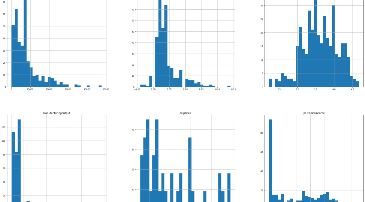
To start with, let us plot the histograms to see the range of each feature and how varies. This will give us an idea of the distribution of the data.
data.hist(figsize=(30, 40), bins=30)array([[<matplotlib.axes._subplots.AxesSubplot object at 0x000001DAE01B5FD0>,
<matplotlib.axes._subplots.AxesSubplot object at 0x000001DAE089F4F0>,
<matplotlib.axes._subplots.AxesSubplot object at 0x000001DAE08CF940>],
[<matplotlib.axes._subplots.AxesSubplot object at 0x000001DAE08FADC0>,
<matplotlib.axes._subplots.AxesSubplot object at 0x000001DAE0935250>,
<matplotlib.axes._subplots.AxesSubplot object at 0x000001DAE095F5E0>],
[<matplotlib.axes._subplots.AxesSubplot object at 0x000001DAE095F6D0>,
<matplotlib.axes._subplots.AxesSubplot object at 0x000001DAE098AB80>,
<matplotlib.axes._subplots.AxesSubplot object at 0x000001DAE09F03D0>],
[<matplotlib.axes._subplots.AxesSubplot object at 0x000001DAE0A1E820>,
<matplotlib.axes._subplots.AxesSubplot object at 0x000001DAE0A48CA0>,
<matplotlib.axes._subplots.AxesSubplot object at 0x000001DAE0A81130>]],
dtype=object)

We can also look for the correlation between these features to figure out which features are more related to each other.
corr = data.corr('pearson')plt.figure(figsize = (15,15))
sns.heatmap(corr, vmax=1.0, vmin=-1.0, square=True, annot=True, annot_kws={"size": 9, "color": "black"},
linewidths=0.1, cmap='rocket')<matplotlib.axes._subplots.AxesSubplot at 0x1dae2835340>
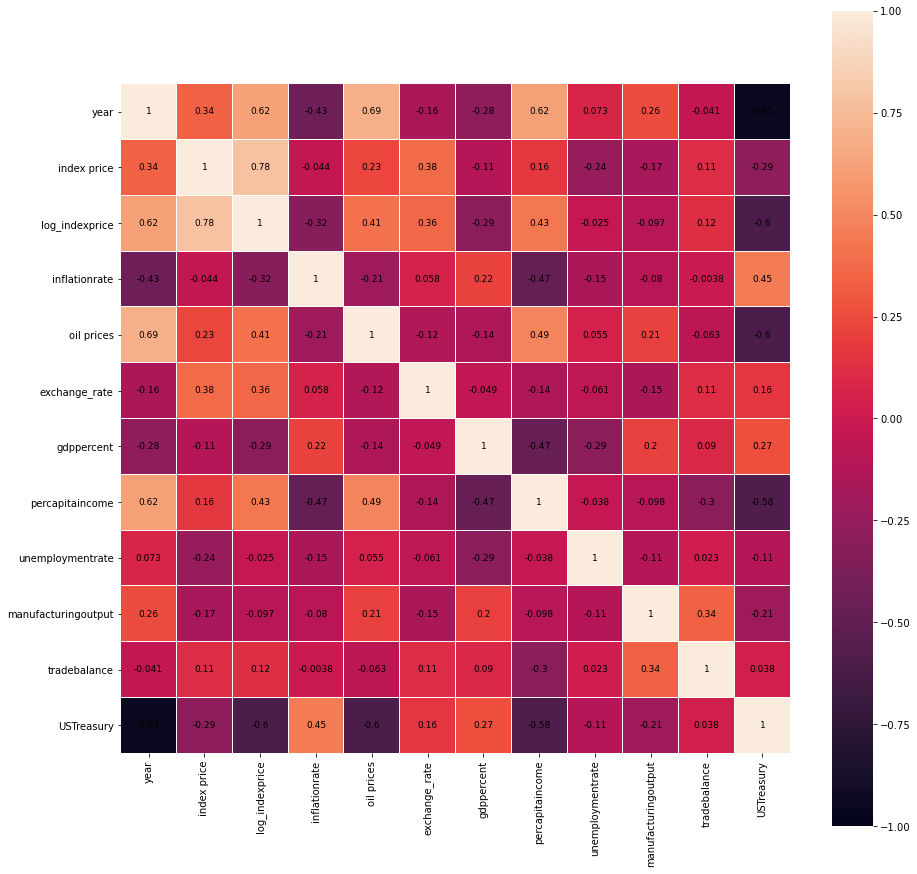
The lighter colours in the heatmap indicate a positive correlation while the darker colours indicate negative correlation. Let us sort these values in descending order to see which features are highly correlated with log_indexprice
corr1 = corr['log_indexprice'].drop(['log_indexprice'])
corr1.sort_values(ascending=False)
index price 0.781482
year 0.618927
percapitaincome 0.431553
oil prices 0.405666
exchange_rate 0.363097
tradebalance 0.119281
unemploymentrate -0.024604
manufacturingoutput -0.097482
gdppercent -0.293933
inflationrate -0.317428
USTreasury -0.598548
Name: log_indexprice, dtype: float64
As expected the feature index price is the most correlated with log_indexprice as the latter is just the log value of the former. Additionally, we see that year and percapitaincome are high to moderately correlated with log_indexprice.
We can even plot the highly correlated features. We will consider a threshold of 0.5 for a strong correlation. Of course, you can choose a different threshold as well.
strong_corr = corr1[abs(corr1) >= 0.5].sort_values(ascending=False).index.tolist()
strong_fet = data.loc[:, strong_corr + ['log_indexprice']]
fig, ax = plt.subplots(1, 2, figsize = (15,7))

for i, ax in enumerate(ax):
    if i < len(strong_corr):
        sns.regplot(x=strong_corr[i], y='log_indexprice', data=strong_fet, ax=ax, line_kws={'color': 'red'})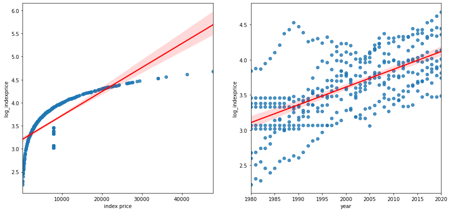
7. Building a Machine Learning Model
Since most features in this dataset are numerical, a Regression Model would be best suited for the scenario. We are considering Linear Regression Model for the sake of simplicity. You can try Polynomial Regression as well. The log_indexprice is taken as the dependent variable. For the independent variable, it can be interesting to see if the inflationrate can be used to predict log_indexprice.
We will first convert the data to a NumPy array. It will then be passed to the LinearRegression() method provided by the scikit-learn library.
x = np.array(data['inflationrate']).reshape((-1, 1))
y = np.array(data['log_indexprice'])
reg = LinearRegression().fit(x, y)
rsquared = reg.score(x, y)
The score() method returns the coefficient of determination of the prediction. It uses the r-squared metric by default.
rsquared0.10076072981661499
8. Conclusion
In this tutorial, we explored the Economic Data of 9 countries. We began with Exploratory Data Analysis and then moved to some basic Visualization. This helped us know more about the correlation among different features. Furthermore, we built a Linear Regression Model where we used the r-squared error metric to determine the goodness of the model.
The error came out to be 0.1 which is decent for a start. However, for future improvements, we can build a Polynomial Regression Model which takes in highly correlated variables. This dataset is comprised of macroeconomic factors and can thus, serve an important purpose for the administrative departments.
Lastly, GridDB made it easier for us to access the data because of its efficient structure
9. References
https://www.kaggle.com/datasets/pratik453609/economic-data-9-countries-19802020 https://www.kaggle.com/code/pratik453609/exploratory-analysis-on-economic-dataset-1980-2020 https://www.kaggle.com/code/algoholiccreations/preliminary-eda-on-economic-dataset-1980-2020
If you have any questions about the blog, please create a Stack Overflow post here https://stackoverflow.com/questions/ask?tags=griddb .
Make sure that you use the “griddb” tag so our engineers can quickly reply to your questions.